Download
1 / 57
570 likes | 715 Views
PRODUCTION AND ITS COSTS. Principles of Microeconomic Theory, ECO 284 John Eastwood CBA 213 523-7353 e-mail address: John.Eastwood@nau.edu http://jan.ucc.nau.edu/~jde. ALL ABOUT COSTS. Explicit and Implicit Costs Accounting Profit and Economic Profit Sunk Costs.

E N D
PRODUCTION AND ITS COSTS • Principles of Microeconomic Theory, ECO 284 • John Eastwood • CBA 213 • 523-7353 • e-mail address: John.Eastwood@nau.edu • http://jan.ucc.nau.edu/~jde
ALL ABOUT COSTS • Explicit and Implicit Costs • Accounting Profit and Economic Profit • Sunk Costs
Explicit and Implicit Costs • Explicit Costs An explicit cost is incurred when an actual monetary payment is made. • Implicit Costs Implicit costs are the value of the resources used in the production of a good for which no monetary payment is made.
Accounting Profit and Economic Profit • Accounting Profit = Total Revenue - total explicit costs • Economic Profit = Total Revenue - opportunity costs • Opportunity Costs= Explicit costs + Implicit costs
Normal Profit • When a firm's revenue just covers its opportunity costs, it is earning a zero economic profit. • This is also known as a normal profit. • Total Cost (TC) includes all opportunity costs, including a normal profit.
Sunk Costs • Costs incurred in the past that cannot be changed by current decisions and cannot be recovered are said to be "sunk."
PRODUCTION AND COSTS IN THE SHORT RUN • The Short-Run Production Function • Inputs And Costs In The Short Run • Total, Average and Marginal Costs
Production Functions • . . . express the relationship between the quantity of the inputs and the maximum quantity of output (q) that can be produced with those inputs. • The quantities of some inputs are variable in the short run (e.g., labor, materials) • The quantity of other inputs (e.g., capital, land) are fixed in the short run.
Short-Run Production Function (a.k.a. TPL) • . . . expresses the relationship between the quantity of the labor and the maximum quantity of output (q) that can be produced, holding the quantity of other inputs (e.g., capital, land) constant.
Example:q=Sand Output (Tons/Day) L=Labor (8-hr. worker-shifts/day)
Table 1: q= Sand (Tons/Day) L=Labor (8-hr. worker-shifts/Day)
Table 1: q= Sand (Tons/Day) L=Labor (8-hr. worker-shifts/Day)
The Average - Marginal Rule • When the marginal magnitude (e.g. product, cost, or utility) exceeds the average magnitude, the average must rise. • When the marginal magnitude is less than the average magnitude, the average must fall. • Marginal curve intersects average curve at a maximum or minimum.
From Definitions to Cost Curves • The Law of Diminishing Marginal Returns • As more units of a variable input are combined with fixed inputs, eventually the marginal physical product of the variable input will decline.
Inputs And Costs In The Short Run • Fixed And Variable Inputs • Fixed and Variable Costs • Total Cost = Total Fixed Cost + Total Variable Cost • TC= TFC + TVC
Example: w=wage; q= Sand (Tons/Day); L=Labor (8-hr. worker-shifts /Day) w = $50/worker-shift TVC = wL($/day) TFC = $100/day TC = TFC + TVC
Example: w=wage; q= Sand (Tons/Day); L=Labor (8-hr. worker-shifts /Day) w = $50/worker-shift TVC = wL($/day) TFC = $100/day TC = TFC + TVC
Example: w=wage; q= Sand (Tons/Day); L=Labor (8-hr. worker-shifts /Day) w = $50/worker-shift TVC = wL($/day) TFC = $100/day TC = TFC + TVC
Average Cost Concepts • Average Fixed Cost, AFC=TFC/q • Average Variable Cost, AVC=TVC/q • Average Total Cost, ATC=TC/q • where q = the quantity of output.
Marginal Cost, MC: • The change in total cost that results from a one unit change in output.
Example: w=wage; q= Sand (Tons/Day); L=Labor (8-hr. worker-shifts /Day)
Example: w=wage; q= Sand (Tons/Day); L=Labor (8-hr. worker-shifts /Day)
Average - Marginal Rule (Again) • When the marginal magnitude exceeds the average magnitude, the average must rise. • When the marginal magnitude is less than the average magnitude, the average must fall. • MC cuts AVC and ATC at their lowest points.
Total Costs Shown as Areas • TC at a given quantity, q, equals the area of the rectangle formed by the origin, q, and ATCq (along both the y-axis and on the curve. • Rectangles formed by AVC and AFC at q show TVC and TFC.
AVC and APPL are Related • As APPL rises, AVC decreases; as APPL falls, AVC increases. Assume labor is the only variable input:
Diminishing Marginal Returns and Marginal Cost • MC and MPP are related. As MPP rises, MC decreases; as MPP falls, MC increases.Assume labor is the only variable input:
PRODUCTION AND COSTS IN THE LONG RUN • Least-cost production • Long run average (total) cost. • Returns to Scale • Economies of Scope • Technological Change
Equal MPP per Dollar • In the long run, all inputs may vary. For example, K may be substituted for L. • Least-cost production requires that each resource is equally productive at the margin:
The Long-Run Average Total Cost Curve (LRATC) • Each possible plant size has a unique short-run ATC curve. • LRATC shows the lowest average cost at which the firm can produce any given level of output.
How LRATC Changes with the Scale of the Firm • Economies of Scale (a.k.a. Increasing returns to scale) LRATC has a negative slope. • Constant Returns to Scale LRATC has a slope = 0. • Diseconomies of Scale (a.k.a. Decreasing returns to scale) LRATC has a positive slope.
Constant Returns to Scale • Say we double all inputs and get double the output • q = f(K,L), and f(2K,2L)=2q • LRATC=LRTC/q • With w & i constant, LRTC doubles. • LRATC ($/unit) is the same at q and 2q. • This is Constant Returns to Scale, CRS.
Increasing Returns to Scale • Say we double all inputs and get more than twice the output • q = f(K,L), but f(2K,2L)>2q • With w & i constant, LRTC doubles. • Output more than doubles. • LRATC = LRTC/q ($/unit) falls • This is Increasing Returns to Scale, IRS (a.k.a. Economies of Scale)
Decreasing Returns to Scale • Say we double all inputs, but get less than twice the output • q = f(K,L), but f(2K,2L)<2q • With w & i constant, LRTC doubles. • But output less than doubles. • LRATC = LRTC/q ($/unit) rises • This is Decreasing returns to scale (a.k.a. Diseconomies of Scale )
LRATC is the Planning Curve • Optimum Plant Size • What is the most efficient scale of operations? • Minimum Efficient Scale • What is the smallest plant that will be competitive?
COST CURVES SHIFT WHEN • Input prices change • The production function shifts • Technological progress occurs • The quantity of fixed inputs changes • Taxes change
Input Prices • Higher prices for fixed inputs shift TFC, TC, AFC, and ATC up. • Higher prices for variable inputs shift TVC, TC, AVC, ATC, and MC up.
Technological progress affects costs in two ways: • It may improve the production process • It may lower input prices
Taxes • . . . on fixed inputs • . . . on variable inputs, output, revenue, profit, etc.
Isocosts and Isoquants • Isocost means one cost. • Isocost lines are similar to budget lines. • Isoquant means one quantity. • Isoquants are similar to indifference curves.
Isocost lines show bundles of (L,K) of equal cost • Let TC = Total Cost • L = quantity of L • w= price of L • K = quantity of K • k= price of K • The y-intercept equals: • The slope equals the relative price of L($/unit L)/ ($/unit K)= units of K per unit of L
Changes in the Isocost Line • Increases in TC shift the Isocost out. • The vertical intercept increases when TC increases. • Changes in relative factor prices rotate the budget line. The slope equals the relative price of L (w/k) . A lower w yields a smaller |slope|.
Isoquant Curves • One isoquant through each point. • Each isoquant slopes down to the right. • Isoquants further from the origin show higher quantities of output. • Isoquants never cross. • Isoquants are bowed toward the origin.
Slope of an Isoquant • at a point equals - MRTSLK • MRTSLK is the Marginal Rate of Technical Substitution of K for L. • MRTSLK = # of units of K the firm must add to replace one unit of L.
Least-Cost Production • . . . occurs once the firm reaches the lowest possible isocost attainable given its output goal. • At that point, the slopes of the isocost and the isoquant are equal.
Equal MPP per Dollar • The tangency of the Isocost and the Isoquant imply that K and L are equally efficient at the margin.
Diminishing Returns (Again) • In Figure 11, on page 189, illustrates this concept using isoquants. • K is fixed in the SR, • As more L is added, the MPPL eventually falls.
q TPnew q2 q1 0 L L2 L1 Product and Process Technology • Better product technology results in new or improved products. • Better process technology shifts the production function upward. TPold
q TPnew q2 q1 0 L L2 L1 Factors that shift TP up • Better process technology. • More of the fixed factors of production. • Workers’ skills improved. TPold