Download
1 / 40
890 likes | 2.83k Views
GIS Data Structures. From the 2-D Map to 1-D Computer Files. Representing Geographic Features: review from opening lecture. How do we describe geographical features? by recognizing two types of data : Spatial data which describes location (where)

E N D
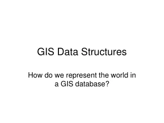
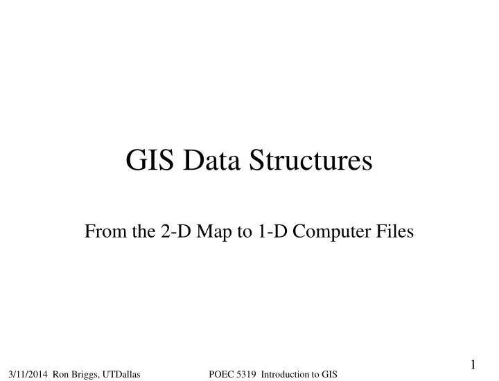
GIS Data Structures From the 2-D Map to 1-D Computer Files
Representing Geographic Features:review from opening lecture How do we describe geographical features? • by recognizing two types of data: • Spatial data which describes location (where) • Attribute data which specifies characteristics at that location (what, how much, and when) How do we represent these digitally in a GIS? • by grouping into layers based on similar characteristics (e.g hydrography, elevation, water lines, sewer lines, grocery sales) and using either: • vector data model (coverage in ARC/INFO, shapefile in ArcView) • raster data model (GRID or Image in ARC/INFO & ArcView) • by selecting appropriate data properties for each layerwith respect to: • projection, scale, accuracy, and resolution How do we incorporate into a computer application system? • by using a relational Data Base Management System (DBMS) We introduced these concepts in the opening lecture. We will deal with them in more detail tonight (except for data properties which will be dealt with under Data Quality).
raster data structures: represents geography via grid cells tesselations run length compression quad tree representation BSQ/BIP/BIL DBMS representation File formats vector data structures:represents geography via coordinates whole polygon point and polygon node/arc/polygon Tins File formats GIS Data Structures: Topics Overview • Spatial data types and Attribute data types • Relational database management systems (RDBMS): basic concepts • DBMS and Tables • Relational DBMS • Overview: representation of surfaces
Spatial Data Types • continuous: elevation, rainfall, ocean salinity • areas: • unbounded: landuse, market areas, soils, rock type • bounded: city/county/state boundaries, ownership parcels, zoning • moving: air masses, animal herds, schools of fish • networks: roads, transmission lines, streams • points: • fixed: wells, street lamps, addresses • moving: cars, fish, deer
Categorical (name): nominal no inherent ordering land use types, county names ordinal inherent order road class; stream class often coded to numbers eg SSN but can’t do arithmetic Numerical Known difference between values interval No natural zero can’t say ‘twice as much’ temperature (Celsius or Fahrenheit) ratio natural zero ratios make sense (e.g. twice as much) income, age, rainfall may be expressed as integer [whole number] or floating point [decimal fraction] Attribute data types Attribute data tables can contain locational information, such as addresses or a list of X,Y coordinates. ArcView refers to these as event tables. However, these must be converted to true spatial data (shape file), for example by geocoding, before they can be displayed as a map.
Data Base Management Systems (DBMS) ContainTablesorfeature classesin which: • rows: entities, records, observations, features: • ‘all’ information about one occurrence of a feature • columns: attributes, fields, data elements, variables, items (ArcInfo) • one type of information for all features The key field is an attribute whose values uniquely identify each row entity Attribute Key field
Relational DBMS: Tables are related, or joined, using a common record identifier(column variable), present in both tables, called a secondary (or foreign) key, which may or may not be the same as the key field. Goal: produce map of values by district/ neighborhood Problem: no district code available in Parcel Table Secondary or foreign key Solution: join Parcel Table, containing values, with Geograpahy Table, containing location codings, using Block as key field
Raster data model location is referenced by a grid cell in a rectangular array (matrix) attribute is represented as a single value for that cell much data comes in this form images from remote sensing (LANDSAT, SPOT) scanned maps elevation data from USGS best for continuous features: elevation temperature soil type land use Vector data model location referenced by x,y coordinates, which can be linked to form lines and polygons attributes referenced through unique ID number to tables much data comes in this form DIME and TIGER files from US Census DLG from USGS for streams, roads, etc census data (tabular) best for features with discrete boundaries property lines political boundaries transportation GIS Data Models: Raster v. Vector“raster is faster but vector is corrector” Joseph Berry
Concept of Vector and Raster Real World Raster Representation Vector Representation point line polygon
area is covered by grid with (usually) equal-sized cells location of each cell calculated from origin of grid: “two down, three over” cells often called pixels (picture elements); raster data often called image data attributes are recorded by assigning each cell a single value based on the majority feature (attribute) in the cell, such as land use type. easy to do overlays/analyses, just by ‘combining’ corresponding cell values: “yield= rainfall + fertilizer” (why raster is faster, at least for some things) simple data structure: directly store each layer as a single table (basically, each is analagous to a “spreadsheet”) computer data base management system not required (although many raster GIS systems incorporate them) 0 1 2 3 4 5 6 7 8 9 1 1 1 1 1 4 4 5 5 5 0 1 1 1 1 1 4 4 5 5 5 1 1 1 1 1 1 4 4 5 5 5 2 1 1 1 1 1 4 4 5 5 5 3 1 1 1 1 1 4 4 5 5 5 4 2 2 2 2 2 2 2 3 3 3 5 2 2 2 2 2 2 2 3 3 3 6 2 2 2 2 2 2 2 3 3 3 7 2 2 4 4 2 2 2 3 3 3 8 2 2 4 4 2 2 2 3 3 3 9 corn fruit wheat clover fruit Representing Data using Raster Model oats
Raster Data Structures: Concepts • grid often has its origin in the upper left but note: • State Plane and UTM, lower left • lat/long & cartesian, center • single values associated with each cell • typically 8 bits assigned to values therefore 256 possible values (0-255) • rules needed to assign value to cell if object does not cover entire cell • majority of the area (for continuous coverage feature) • value at cell center • ‘touches’ cell (for linear feature such as road) • weighting to ensure rare features represented • choose raster cell size 1/2 the length (1/4 the area) of smallest feature to map (smallest feature called minimum mapping unit or resel--resolution element) • raster orientation: angle between true north and direction defined by raster columns • class: set of cells with same value (e.g. type=sandy soil) • zone: set of contiguous cells with same value • neighborhood: set of cells adjacent to a target cell in some systematic manner
Square grid: equal length sides conceptually simplest cells can be recursively divided into cells of same shape 4-connected neighborhood (above, below, left, right) (rook’s case) all neighboring cells are equidistant 8-connected neighborhood (also include diagonals) (queen’s case) all neighboring cells not equidistant center of cells on diagonal is 1.41 units away (square root of 2) rectangular commonly occurs for lat/long when projected data collected at 1degree by 1 degree will be varying sized rectangles triangular (3-sided) and hexagonal (6-sided) all adjacent cells and points are equidistant triangulated irregular network (tin): vector model used to represent continuous surfaces (elevation) more later under vector Raster Data Structures: Tesselations(Geometrical arrangements that completely cover a surface.)
Full Matrix--162 bytes 111111122222222223 111111122222222233 111111122222222333 111111222222223333 111113333333333333 111113333333333333 111113333333333333 111333333333333333 111333333333333333 1,7,2,17,3,18 1,7,2,16,3,18 1,7,2,15,3,18 1,6,2,14,3,18 1,5,3,18 1,5,3,18 1,5,3,18 1,3,3,18 1,3,3,18 Raster Data StructuresRunlength Compression (for single layer) Run Length (row)--44 bytes This is a “lossless” compression, as opposed to “lossy,” since the original data can be exactly reproduced. Now, GIS packages generally rely on commercial compression routines. Pkzip is the most common, general purpose routine. MrSid (from Lizard Technology)and ECW (from ER Mapper) are used for images. All these essentially use the same concept. Occasionally, data is still delivered to you in run-length compression, especially in remote sensing applications. “Value thru column” coding. 1st number is value, 2nd is last column with that value.
sides of square grid divided evenly on a recursive basis length decreases by half # of areas increases fourfold area decreases by one fourth Resample by combining (e.g. average) the four cell values although storage increases if save all samples, can save processing costs if some operations don’t need high resolution for nominal or binary data can save storage by using maximum block representation all blocks with same value at any one level in tree can be stored as single value 1 1 1 1 1 1 Raster Data StructuresQuad Tree Representation (for single layer) Essentially involves compression applied to both row and column. 3.25 3 4 3.5 2.5 2 4 5 3 4 2 4 4 4 4 1 4 2 4 3 2 store this quadrant as single 1 1 1 store this quadrant as single zero I 1,0,1,1 II 1 III 0,0,0,1 IV 0
raster data comprises rows and columns, by one or more characteristics or arrays elevation, rainfall, & temperature; or multiple spectral channels (bands) for remote sensed data how organise into a one dimensional data stream for computer storage & processing? Band Sequential (BSQ) each characteristic in a separate file elevation file, temperature file, etc. good for compression good if focus on one characteristic bad if focus on one area Band Interleaved by Pixel (BIP) all measurements for a pixel grouped together good if focus on multiple characteristics of geographical area bad if want to remove or add a layer Band Interleaved by Line (BIL) rows follow each other for each characteristic B B A B III IV I II 150 160 120 140 Raster Data Structures: Raster Array Representations for multiple layers Veg Soil Elevation Note that we start in lower left. Upper left is alternative. File 1: Veg A,B,B,B File 2: Soil I,II,III,IV File 3: El. 120,140,150,160 A,I,120, B,II,140 B,III,150 B,IV,160 A,B,I,II,120,140 B,B,III,IV,150,160
raw data may come in BSQ, BIP, BIL but not good for efficient for GIS processing Can be represented as standard data base table joins based on ID as the key field can be used to relate variables in different tables Raster Data StructuresDatabase Representation
File Formats for Raster Spatial Data The generic raster data model is actually implemented in several different computer file formats: • GRID is ESRI’s proprietary format for storing and processing raster data • Standard industry formats for image data such as JPEG, TIFF and MrSid formats can be used to display raster data, but not for analysis (must convert to GRID) • Georeferencing information required to display images with mapped vector data (will be discussed later in course) • Requires an accompanying “world” file which provides locational information Image I mage File World File TIFF image.tif image.tfw Bitmap image.bmp image.bpw BIL image.bil image.blw JPEG image.jpg image.jpw Although not commonly encountered, a “geotiff’ is a single file which incorporates both the image and the “world” information is a single file.
2 2 1 1 1 7 7 8 8 2 1 7 8 2 1 7 8 Vector Data Model Representing Data using the Vector Model:formal application . • point (node): 0-dimension • single x,y coordinate pair • zero area • tree, oil well, label location • line (arc): 1-dimension • two (or more) connected x,y coordinates • road, stream • polygon : 2-dimensions • four or more ordered and connected x,y coordinates • first and last x,y pairs are the same • encloses an area • census tracts, county, lake y=2 Point: 7,2 x=7 Line: 7,2 8,1 Polygon: 7,2 8,1 7,1 7,2
Vector Data Structures: Whole Polygon Whole Polygon (boundary structure): polygons described by listing coordinates of points in order as you ‘walk around’ the outside boundary of the polygon. • all data stored in one file • could also store--inefficiently--attribute data for polygon in same file • coordinates/borders for adjacent polygons stored twice; • may not be same, resulting in slivers (gaps), or overlap • how assure that both updated? • all lines are ‘double’ (except for those on the outside periphery) • no topological information about polygons • which are adjacent and have common boundary? • how relate different geographies? e.g. zip codes and tracts? • used by the first computer mapping program, SYMAP, in late ‘60s • adopted by SAS/GRAPH and many business thematic mapping programs. Topology --knowledge about relative spatial positioning --managing data cognizant of shared geometry Topography --the form of the land surface, in particular, its elevation
A 3 4 A 4 4 A 4 2 A 3 2 A 3 4 B 4 4 B 5 4 B 5 2 B 4 2 B 4 4 C 3 2 C 4 2 C 4 0 A B E C D Whole Polygon:illustration Data File C 3 0 C 3 2 D 4 2 D 5 2 D 5 0 D 4 0 D 4 2 E 1 5 E 5 5 E 5 4 E 3 4 E 3 0 E 1 0 E 1 5 5 4 3 2 1 0 1 2 3 4 5
Vector Data Structures: Points & Polygons Points and Polygons: polygons described by listing ID numbers of points in order as you ‘walk around the outside boundary’; a second file lists all points and their coordinates. • solves the duplicate coordinate/double border problem • lines can be handled similar to polygons (list of IDs) , but how handle networks? • still no topological information • first used by CALFORM, the second generation mapping package, from the Laboratory for Computer Graphics and Spatial Analysis at Harvard in early ‘70s
1 3 4 2 4 4 3 4 2 4 3 2 5 5 4 6 5 2 7 5 0 8 4 0 9 3 0 10 1 0 11 1 5 12 5 5 Points and Polygons:Illustration Points File Polygons File 12 A 1, 2, 3, 4, 1 B 2, 5, 6, 3, 2 C 4, 3, 8, 9, 4 D 3, 6, 7, 8, 3 E 11, 12, 5, 1, 9, 10, 11 5 11 2 5 1 4 3 A B E 3 4 6 2 C D 1 10 9 8 7 0 1 2 3 4 5
Vector Data Structure: Node/Arc/Polygon Topology Comprises 3 topological components which permit relationships between all spatial elements to be defined (note: does not imply inclusion of attribute data) • ARC-node topology: • defines relations between points, by specifying which are connected to form arcs • defines relationships between arcs (lines), by specifying which arcs are connected to form routes and networks • Polygon-Arc Topology • defines polygons (areas) by specifying which arcs comprise their boundary • Left-Right Topology • defines relationships between polygons (and thus all areas) by • defining from-nodes and to-nodes, which permit • left polygon and right polygon to be specified • ( also left side and right side arc characteristics) Left from Right to
II 1 2 Birch Node/Arc/ Polygon and Attribute Data Relational Representation: DBMS required! Smith Estate I A34 III A35 4 IV 3 Cherry Attribute Data Spatial Data
1 5 4 2 3 X Representing Point Data using the Vector Model:data implementation • Features in the theme (coverage) have unique identifiers--point ID, polygon ID, arc ID, etc • common identifiers provide link to: • coordinates table (for ‘where) • attributes table (for what) Y • Again, concepts are those of a relational data base, which is really a prerequisite for the vector model
TIN: Triangulated Irregular Network Surface Polygons Attribute Info. Database Points Elevation points (nodes) chosen based on relief complexity, and then their 3-D location (x,y,z) determined. Elevation points connected to form a set of triangular polygons; these then represented in a vector structure. Attribute data associated via relational DBMS (e.g. slope, aspect, soils, etc.) 2 1 E A B 3 • Advantages over raster: • fewer points • captures discontinuities (e.g ridges) • slope and aspect easily recorded • Disadvans.: Relating to other polygons for map overlay is compute intensive (many polygons) D C 4 F G 5 6 H
File Formats for Vector Spatial Data Generic models above are implemented by software vendors in specific computer file formats Coverage:vector data format introduced with ArcInfo in 1981 • multiple physical files (12 or so) in a folder • proprietary: no published specs & ArcInfo required for changes Shape ‘file’:vector data format introduced with ArcView in 1993 • comprises several (at least 3) physical disk files (with extension of .shp, .shx, .dbf), all of which must be present • openly published specs so other vendors can create shape files Geodatabase: new format introduced with ArcGIS 8.0 in 2000 • Multiple layers saved in a singe .mdb (MS Access-like) file • Proprietary, “next generation” spatial data file format Shapefiles are the simplest and most commonly used format and will generally be used in the class exercises.
Geographic Data: Another Perspective Object View • The real world is a series of entities located in space. • An object is a digital representation of an entity, with three types • Point objects • Line objects • Area objects • The same entity can be represented at different scales by different object types: multi-representation • Behavior can be associated with objects thus they can change over time Field View • The real world has properties which vary continuously over space; every place has a value • May be represented as raster data, or with vector data as a TIN (triangulated irregular network Field or Object? • If the field value is a categorical or integer variable, then places with the same value (e.g. crop type) can be grouped---into area objects?! 1 1 1 1 1 4 4 5 5 5 corn 1 1 1 1 1 4 4 5 5 5 fruit 1 1 1 1 1 4 4 5 5 5 1 1 1 1 1 4 4 5 5 5 1 1 1 1 1 4 4 5 5 5 2 2 2 2 2 2 2 3 3 3 wheat clover 2 2 2 2 2 2 2 3 3 3 2 2 2 2 2 2 2 3 3 3 2 2 4 4 2 2 2 3 3 3 fruit 2 2 4 4 2 2 2 3 3 3 The world is how we decide to look at it!!! From O’Sullivan and Unwin Geographic Information Analysis, Wiley, 2003 Useful perspective since it parallels object oriented concepts in software technology.
Tongariro National Park North Island New Zealand Representing Surfaces
z x y Overview: Representing Surfaces • Surfaces involve a third elevation value (z) in addition to the x,y horizontal values • Surfaces are complex to represent since there are an infinite number of potential points to model • Three (or four) alternative digital terrain modelapproaches available • Raster-based digital elevation model • Regular spaced set of elevation points (z-values) • Vector based triangulated irregular networks • Irregular triangles with elevations at the three corners • Vector-based contour lines • Lines joining points of equal elevation, at a specified interval • Massed points and breaklines • The raw data from which one of the other three is derived • Massed points: Any set of regular or irregularly spaced point elevations • Breaklines: point elevations along a line of significant change in slope (valley floor, ridge crest)
Digital Elevation Model • Advantages • Simple conceptual model • Data cheap to obtain • Easy to relate to other raster data • Irregularly spaced set of points can be converted to regular spacing by interpolation • Disadvantages • Does not conform to variability of the terrain • Linear features not well represented • a sampled array of elevations (z) that are at regularly spaced intervals in the x and y directions. • two approaches for determining the surface z value of a location between sample points. • In a lattice, each mesh point represents a value on the surface only at the center of the grid cell. The z-value is approximated by interpolation between adjacent sample points; it does not imply an area of constant value. • A surface grid considers each sample as a square cell with a constant surface value.
Triangulated Irregular Network a set of adjacent, non-overlapping triangles computed from irregularly spaced points, with x, y horizontal coordinates and z vertical elevations. • Advantages • Can capture significant slope features (ridges, etc) • Efficient since require few triangles in flat areas • Easy for certain analyses: slope, aspect, volume • Disadvantages • Analysis involving comparison with other layers difficult
valley hilltop ridge Contour (isolines) Lines Contour lines, or isolines, of constant elevation at a specified interval, Advantages • Familiar to many people • Easy to obtain mental picture of surface • Close lines = steep slope • Uphill V = stream • Downhill V or bulge = ridge • Circle = hill top or basin Disadvantages • Poor for computer representation: no formal digital model • Must convert to raster or TIN for analysis • Contour generation from point data requires sophisticated interpolation routines, often with specialized software such as Surfer from Golden Software, Inc., or ArcGIS Spatial Analyst extension
Appendix GIS File Formats Some additional detail
Vendor Implementation of GIS Data Structures:file formats • Raster, vector, TIN, etc. are generic models for representing spatial information in digital form • GIS vendors implement these models in file formats or structures which may be • Proprietary: useable only with that vendor’s software (e.g. ESRI coverage) • Published: specifications available for use by any vendor (e.g ESRI shapefile, or the military vpf format) • Transfer formats: intended only for transfer of data • Between different vendor’s systems (e.g. AutoCAD .dxf format, or SDTS) • between different users of same vendors’ software (e.g. ESRI’s E00 format for coverages) • One GIS vendor may be able to read another file format: • By translation, whereby format is converted externally to vendors own format • Usually requires user to carry out conversion prior to use of data • On-the-fly, whereby conversion is accomplished internally and “automatically” • No user action needed, but usually no ability to change data • Natively, or transparently, which normally implies • No special user action needed • ability to read and write (change or edit) the data best
ESRI Coverages (vector--proprietary) E00 (“E-zero-zero”) for coverage exchange between ESRI users Shapefiles (vector--published) .shp Geodatabase (proprietary) .gdb Based on current object-oriented software technology GRID (raster) AutoCAD AutoCAD .DWG (native) AutoCAD .DXF for digital file exchange Intergraph/Bentley Bentley MicroStation .DGN Intergraph/Bentley .MGE Common GIS & CAD File Formats • Spatial Data Transfer Standard (SDTS) • US federal standard for transfer of data • Federal agencies legally required to conform • embraces the philosophy of self-contained transfers, i.e. spatial data, attribute, georeferencing, data quality report, data dictionary, and other supporting metadata all included • Not widely adopted ‘cos of competitive pressures, and complexity and perceived disutility derived from philosophy
Shape ‘file’:native GIS data structure for a vector layer in ArcView not fully topological limited info about relationship of features one to another draw faster not as good for some fancy spatial analyses is a ‘logical’ file which comprises several (at least 3) physical disk files, all of which must be present for AV to read the theme layer.shp (geometric shape described by XY coords) layer.shx (indices to improve performance) layer.dbf (contains associated attribute data) layer.sbn layer.sbx not really a database, although ArcView presents files to user via relational concepts openly published specs so other vendors can develop shape files and read them Coverage:nativeGIS data structure for a vector layer in ArcInfo fully topological better suited for large data sets better suited for fancy spatial analyses comprises multiple physical files (12 or so) per coverage each coverage saved in a separate folder named same as the coverage physical file set differs depending on type of coverage (point, line, polygon). coverage folders stored in a “workspace” directory with an info folder for tracking attribute tables stored there also ARC/INFO required to make changes proprietary: no published specs. E00 Export Files:format for export of coverages to other ESRI users IMPORT71 utility in ArcView Start Menu can read E00 files and convert them back to coverages Must convert to shapefile or AutoCAD .dxf format to transfer to a non-ESRI GIS system ESRI Vector File Formats: “Georelational”
I. Geo-relational Database the old “classic” environment proprietary coverages in ArcInfo (INFO database) published shapefiles in ArcView (dbIV database) Based on points, lines, polygon model II. Geodatabase The new term with ArcInfo 8 in 2000 Replacement for coverages, and support for Simple features: points, lines polygons Complex features: real world entities modeled as objects with properties, behavior, rules, & relationships AV downgrades complex features to simple features Personal Geodatabase Single-user editing Stored as one .mdb file (but Access can’t read) AV 3.2 cannot read (to be “fixed” later) Multiuser Geodatabase Supports versioning and long transactions Uses ArcSDE 8 as middleware Stores in standard db: ORACLE, MS SQL Server, Informix, Sybase, IBM DB2 AV3.2 can read ArcGIS 8 Database Environment
Image files:raster supported in several formats: BSQ, BIL, BIP and run length comp. JPEG (must load JPEG image extension) TIFF (must license a dll if LZW comp. used) ERDAS GIS, LAN, IMAGINE Georeferencing information required if images to be displayed with mapped vector data cells of the raster must be converted to the XY coordinate metric (lat/long, projected feet etc.) of the map stored in header file of the raster image (e.g. GEOTIFF) or in a separate “world” file Image Image File World File TIFF image.tif image.tfw Bitmap image.bmp image.bpw BIL image.bil image.blw Be sure you have both files! GRID: native proprietary format for a raster file in Arc/Info incorporates positioning info. can be read by ArcView all raster-based analyses require files in GRID format, including ArcView Spatial 3-D Analyst ArcView has some limited capabilities for converting to GRID format, but generally this requires ARC/INFO ( or the PC-based Data Automation Kit) when ArcView saves GRID data sets it does so in an ARC/INFO-style format: ArcCatalog must be used to manage these ArcGIS Raster File Formats
ESRI “middleware” product designed to interface with industry-standard RDBMS for large scale spatial data bases First introduced with ArcInfo Version 7 in the mid 1990s;ArcView version 3.0 and later can read SDE both attribute and spatial data is stored in the same RDBMS (such as Oracle, which supports SDE) allows mass data capabilities, security and data integrity mechanisms of the RDBMS to be applied to the spatial data data is grouped into: sets, which share common security (e.g. all data for a city) layers, similar to themes (e.g. road layer, parcel layer) features, individual elements (e.g. single road) advantages for large data sets include layers are not tiled, so no re-assembly is required features can be extracted as a complete element e.g. entire road Spatial Database Engine (SDE) Arcinfo/arcview rdbms sde