Overview of Robust Methods Analysis
270 likes | 547 Views
Overview of Robust Methods Analysis. Jinxia Ma November 7, 2013. Contents. What are robust methods Why robust methods How to conduct the robust methods analysis Apply robust analysis to your data. What are “robust methods”?.

Overview of Robust Methods Analysis
E N D
Presentation Transcript
Overview of Robust Methods Analysis Jinxia Ma November 7, 2013
Contents • What are robust methods • Why robust methods • How to conduct the robust methods analysis • Apply robust analysis to your data
What are “robust methods”? • Robust statistics are statistics with good performance for data drawn from a wide range of probability distributions, especially for distributions that are not normally distributed. • Outliers • Departures from parametric distributions
Why robust methods? • What’s the problem of standard methodologies? • Example: Linear regression assumptions • Linearity • Independence of errors • Errors are normally distributed • Homoscedasticity • Example: comparing groups (ANOVA F-test) • Errors have a common variance, normally distributed and independent
Why robust methods? • Example: Detecting differences among groups • Problem 1: Heavy-tailed distributions Figure 1: Despite the obvious similarity between the standard normal and contaminated normal distributions, the standard normal has variance 1 and the contaminated normal has variance 10.9.
Why robust methods? • Example: Detecting differences among groups • Problem 1: Heavy-tailed distributions Figure 2: Left panel, power = 0.96. Right panel, power = 0.28. (n= 25 per group, Student’s T test.
Why robust methods? • Example: Detecting differences among groups • Problem 1: Heavy-tailed distributions Correlation = .8 Correlation = .2 Correlation = .2 Figure 3: Left panel, a bivariate normal distribution, corr = .8. Middle panel, a bivariate normal distribution, corr= .2. Right panel, one marginal distribution is normal, but the other is a contaminated normal, corr = .2.
Why robust methods? • Example: Detecting differences among groups • Problem 2: Assuming normality via the central limit theorem Figure 4: The distribution of Student’s T, n=25, when sampling from a (standard) lognormal distribution. The dashed line is the distribution under normality. For real Student’s T: P(T<=-2.086)=P(T>=2.086)=.025, E(T)=0. For “Lognormal T”: P(T<=-2.086)=.12, P(T>=2.86)=.001, E(T)=-.54.
Why robust methods? • Example: Detecting differences among groups • Problem 3: Heteroscedasticity • The third fundamental insight is that violating the usual homoscedasticity assumption (i.e. the assumption that all groups are assumed to have a common variance), is much more serious than once thought. Both relatively poor power and inaccurate confidence intervals can result.
How to test/compare robust methods? • Example: Comparing dependent groups with missing values: an approach based on a robust method • 1: Simulation • 2: Bootstrap
How to test/compare robust methods? • Example: Comparing dependent groups with missing values: an approach based on a robust method • 1: Simulation • g-and-h distribution • Let Z be a random variable generated from a standard normal distribution, then W has a g-and-h distribution.
How to test/compare robust methods? • Example: Comparing dependent groups with missing values: an approach based on a robust method • 1: Simulation • g-and-h distribution • g=h=0, standard normal • G>0, skewed; the bigger the value of g, the more skewed. • H>0, heavy-tailed; the bigger the value of h, the more heavy-tailed.
How to test/compare robust methods? • 1: Simulation • g-and-h distribution
How to test/compare robust methods? • 2: Bootstrap (B = 2000)
Robust solutions • Alternate Measures of Location • One way of dealing with outliers is to replace the mean with alternative measures of location • Median • Trimmed mean • Winsorized mean • M-estimator
Robust solutions • Transformations • A simple way of dealing with skewness is to transform the data. • Logarithms • Simple transformations do not deal effectively with outliers • The resulting distributions can remain highly skewed
Robust solutions • Nonparametric regression • Sometimes called smoothers. • Imagine that in a regression situation the goal is to estimate the mean of Y, given that X=6, based on n pairs of observations. The strategy is to focus on the observed X values close to 6 and use the corresponding Y values to estimate the mean of Y. Typically, smoothers give more weight to Y values for which the corresponding X values are close to 6. For pairs of points for which the X value is far from 6, the corresponding Y values are ignored.
Robust solutions • Robust measures of association • Use some analog of Pearson’s correlation that removes or down weights outliers • Fit a regression line and measure the strength of the association based on this fit.
Practical Illustration of Robust Methods • Analysis of a lifestyle intervention for older adults • N=364 • This trial was conducted to compare a six-month lifestyle intervention to a no treatment control condition • Outcome variables: (a) eight indices of health-related quality of life; (b) depression; (c) life satisfaction. • Preliminary analysis revealed that all outcome variables were found to have outliers based on boxplots.
Practical Illustration of Robust Methods • Analysis of a lifestyle intervention for older adults • Figure 5: The median regression line for predicting physical function based on the number of session hours (R function: qsmcobs). • r=.178 (p=.001). However, the association appears to be non-linear.
Practical Illustration of Robust Methods • Analysis of a lifestyle intervention for older adults • Figure 6: The median regression line for predicting physical composite based on the number of session hours (R function: qsmcobs). • For 0 to 5 hours, r=-.071 (p=.257). • For 5 hours or more, r=.25 (p=.045).
Practical Illustration of Robust Methods • Analysis of a lifestyle intervention for older adults Table: Measures of association between hours of treatment and the variables listed in column 1 (n = 364). rw* = 20% Winsorized correlation
Practical Illustration of Robust Methods • Analysis of a lifestyle intervention for older adults Table 2: P-values when comparing ethnic matched group patients to a non-matched group. Welch’s test: dealing with heteroscedasticity Yuen’s test: based on trimmed means No single method is always best.
Software • R: www.r-project.org • www.rcf.usc.edu/~rwilcox • Example: comparing two groups • > x1=read.table(file=“ ”) • > x2=read.table(file=“ ”) • > x<-list(x1,x2) • > lincon(x,tr=0.2,alpha=0.05) • Linconis a heteroscedastictest of d linear contrasts using trimmed means.