Inductive Modeling
In this lecture, we shall study yet more general techniques for identifying complex non-linear models from observations of input/output behavior. These techniques make an attempt at mimicking human capabilities of vicarious learning , i.e., of learning from observation.


Inductive Modeling
E N D
Presentation Transcript
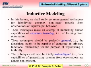
In this lecture, we shall study yet more general techniques for identifying complex non-linear models from observations of input/output behavior. These techniques make an attempt at mimicking human capabilities of vicarious learning, i.e., of learning from observation. These techniques should be perfectly general, i.e., the algorithms ought to be capable of capturing an arbitrary functional relationship for the purpose of reproducing it faithfully. The techniques will also be totally unintelligent, i.e., their capabilities of generalizing patterns from observations are almost non-existent. Inductive Modeling
Knowledge-based vs. observation-based modeling Taxonomy of modeling methodologies Observation-based modeling and optimization Observation-based modeling and complexity Artificial neural networks Parametric vs. non-parametric modeling Quantitative vs. qualitative modeling Fuzzy modeling Fuzzy inductive reasoning Cardiovascular system Table of Contents
Until now, we have almost exclusively embraced modeling techniques that were based on a priori knowledge. Only on a very few occasions have we created models from observations. The one time that we really tried to do this, namely when we created a Lotka-Volterra model of the larch bud moth, we were not overly successful in our endeavor. Yet, when we use a priori knowledge, such as when we model a resistor using the equation: u = R·i, we are not really making models – we are only using models that had been made for us by someone else. Knowledge-based vs. Observation-based Modeling
Knowledge-Based Approaches Observation-Based Approaches Deep Models Shallow Models SD Inductive Reasoners Neural Networks FIR Taxonomy of Modeling Methodologies
Any observation-based modeling methodology is closely linked to optimization. Let us look once more at our Lotka-Volterra models: When we used this structure to model the population dynamics of the larch bud moth, we mapped the observational knowledge available onto the parameters of the Lotka-Volterra equations, i.e., a, b, c, k, xprey0, and xpred0. Modeling here meant to identify these parametervalues, i.e., to minimize the error between the observed and simulated behavior by means of optimization. · Ppred = -a · Ppred + k · b · Ppred · Pprey · Pprey = c· Pprey-b · Ppred · Pprey Observation-based Modeling and Optimization
Observation-based modeling is very important, especially when dealing with unknown or only partially understood systems. Whenever we deal with new topics, we really have no choice, but to model them inductively, i.e., by using available observations. The less we know about a system, the more general a modeling technique we must embrace, in order to allow for all eventualities. If we know nothing, we must be prepared for anything. In order to model a totally unknown system, we must thus allow a model structure that can be arbitrarily complex. Observation-based Modeling and Complexity
One very popular approach to model systems from observations is by use of artificial neural networks (ANNs). ANNs are modeled after the neurons of the human brain. w’is theweight vector + u1 bis thebias u2 y activation()is a non-linearactivation function, usually shaped after the logistic equation, e.g.: … un x = w’ · u + b y = activation(x) 1.0 y = sigmoid(x) = 1.0 + exp(-x) Artificial Neural Networks (ANN) I
Many such neurons are grouped together in a matrix structure: The weight matrices and bias vectors between neighboring network layers store the information about the function to be modeled. u1 + + + + + + + + + + + y u2 Artificial Neural Networks (ANN) II
It can be shown that an ANN with a single hidden layer and enough neurons on it can learn any function with a compact domain of the input variables. With at least two hidden layers, even arbitrary functions with holes in their input domains can be learnt. u3 y3 u2 y2 Input/output map u1 y1 Artificial Neural Networks (ANN) III
ANNs are parametric models. The observed knowledge about the system under study is mapped on the (potentially very large) set of parameters of the ANN. Once the ANN has been trained, the original knowledge is no longer used. Instead, the learnt behavior of the ANN is used to make predictions. This can be dangerous. If the testing data, i.e. the input patterns during the use of the already trained ANN differ significantly from the training data set, the ANN is likely to predict garbage, but since the original knowledge is no longer in use, is unlikely to be aware of this problem. Parametric vs. Non-parametric Models I
Non-parametric models, on the other hand, always refer back to the original training data, and therefore, can be made to reject testing data that are incompatible with the training data set. The Fuzzy Inductive Reasoning(FIR) engine that we shall discuss in this lecture, is of the non-parametric type. During the training phase, FIR organizes the observed patterns, and places them in a data base. During the testing phase, FIR searches the data base for the five most similar training data patterns, the so-called five nearest neighbors, by comparing the new input pattern with those stored in the data base. FIR then predicts the new output as a weighted average of the outputs of the five nearest neighbors. Parametric vs. Non-parametric Models II
Training a model (be it parametric or non-parametric) means solving an optimization problem. In the parametric case, we have to solve a parameter identification problem. In the non-parametric case, we need to classify the training data, and store them in an optimal fashion in the data base. Training such a model can be excruciatingly slow. Hence it may make sense to devise techniques that will help to speed up the training process. Quantitative vs. Qualitative Models I
How can the speed of the optimization be controlled? Somehow, the search space needs to be reduced. One way to accomplish this is to convert continuous variables to equivalent discrete variables prior to optimization. For example, if one of the variables to be looked at is the ambient temperature, we may consider to classify temperature values on a spectrum from very cold to extremely hot as one of the following discrete set: Quantitative vs. Qualitative Models II temperature = { freezing, cold, cool, moderate, warm, hot }
A variable that only assumes one among a set of discrete values is called a discrete variable. Sometimes, it is also called a qualitative variable. Evidently, it must be cheaper to search through a discrete search space than through a continuous search space. The problem with discretization schemes, such as the one proposed above, is that a lot of potentially valuable detailed information is being lost in the process. To avoid this pitfall, L. Zadeh proposed a different approach, called fuzzification. Qualitative Variables
Fuzzification proceeds as follows. A continuous variable is fuzzified, by decomposing it into a discrete class value and a fuzzy membership value. For the purpose of reasoning, only the class value is being considered. However, for the purpose of interpolation, the fuzzy membership value is also taken into account. Fuzzy variables are not discrete, but they are also referred to as qualitative. Fuzzy Variables I
Systolic blood pressure = 141 { normal, 0.78 } { too high, 0.18 } Systolic blood pressure = 110 { normal, 0.78 } { too low, 0.15 } Fuzzy Variables II { Class, membership } pairs of lower likelihood must be considered as well, because otherwise, the mapping would not be unique.
right left Systolic blood pressure = 110 Systolic blood pressure = 141 { normal, 0.78, left } { normal, 0.78, right } Fuzzy Variables in FIR FIR embraces a slightly different approach to solving the uniqueness problem. Rather than mapping into multiple fuzzy rules, FIR only maps into a single rule, that with the largest likelihood. However, to avoid the aforementioned ambiguity problem, FIR stores one more piece of information, the “side value.” It indicates, whether the data point is to the left or the right of the peak of the fuzzy membership value of the given class.
Neural Networks Fuzzy Inductive R. Neural Networks vs. Inductive Reasoners
Discretization of quantitative information (Fuzzy Recoding) Reasoning about discrete categories (Qualitative Modeling) Inferring consequences about categories (Qualitative Simulation) Interpolation between neighboring categories using fuzzy logic (Fuzzy Regeneration) Fuzzy Inductive Reasoning (FIR) I
FIR Crisp data Crisp data Fuzzy Recoding Regene- ration Fuzzy Modeling Fuzzy Simulation Fuzzy Inductive Reasoning (FIR) II
Once the data have been recoded, we wish to determine, which among the possible set of input variables best represents the observed behavior. Of all possible input combinations, we pick the one that gives us as deterministic an input/output relationship as possible, i.e., when the same input pattern is observed multiple times among the training data, we wish to obtain output patterns that are as consistent as possible. Each input pattern should be observed at least five times. Qualitative Modeling in FIR I
Fuzzy rule base y1(t) = f ( y3(t-2t), u2(t-t) , y1(t-t) , u1(t) ) Qualitative Modeling in FIR II
Qualitative Modeling in FIR III • The qualitative model is the optimal mask, i.e., the set of inputs that best predict a given output. • Usually, the optimal mask is dynamic, i.e., the current output depends both on current and past values of inputs and outputs. • The optimal mask can then be applied to the training data to obtain a set of fuzzy rules that can be alphanumerically sorted. • The fuzzy rule base is our training data base.
Behavior Matrix Raw Data Matrix 2 Input Pattern Optimal Mask 2 3 Matched Input Patterns 1 3 Euclidean Distance Computation dj 1 1 ? 5-Nearest Neighbors Output Computation fi=F(W*5-NN-out) Class Forecast Value Membership Side Qualitative Simulation in FIR
Time-series Prediction in FIR Water demand for the city of Barcelona, January 85 – July 86
Prediction Real Simulation Results I
Deductive Modeling Techniques * have a large degree of validity in many different and even previously unknown applications * are often quite imprecise in their predictions due to inherent model inaccuracies Inductive Modeling Techniques * have a limited degree of validity and can only be applied to predicting behavior of systems that are essentially known * are often amazingly precise in their predictions if applied carefully Quantitative vs. Qualitative Modeling
Quantitative Subsystem Quantitative Subsystem FIR Model FIR Model Recode Recode Regenerate Regenerate Mixed Quantitative & Qualitative Modeling • It is possible to combine qualitative and quantitative modeling techniques.
Application: Cardiovascular System I • Let us apply the technique to a fairly complex system: the cardiovascular system of the human body. • The cardiovascular system is comprised of two subsystems: the hemodynamic system and the central nervous control. • The hemodynamic system describes the flow of blood through the heart and the blood vessels. • The central nervous control synchronizes the control algorithms that control the functioning of both the heart and the blood vessels.
Application: Cardiovascular System II • The hemodynamic system is essentially a hydrodynamic system. The heart and blood vessels can be described by pumps and valves and pipes. Thus bond graphs are suitable for its description. • The central nervous control is still not totally understood. Qualitative modeling on the basis of observations may be the tool of choice.
The Hemodynamic System I The heart chambers and blood vessels are containers of blood. Each container is a storage of mass, thus contains a C-element. The C-elements are partly non-linear, and in the case of the heart chambers even time-dependent. The mSe-element on the left side represents the time-varying pressure caused by the contracting heart. The mSe-element on the right side represents the thoracic pressure, which is influenced by the breathing.
All containers are drawn as boxes. They end in 0-junctions. All flows between containers are drawn as arrows. They end in bonds. As long as containers and flows toggle, they can be connected together without bonds in between. Some of the flows contain inductors, others only resistances. Some of them also contain valves, which are represented by Sw-elements. The Hemodynamic System IV
The Heart The heart contains the four chambers, as well as the four major heart valves, the pulmonary and aorta valves at the exits of the ventricula, and the mitral and triscuspid valves between the atria and the corresponding ventricula. The sinus rhythm block programs the contraction and relaxation of the heart muscle. The heart muscle flow symbolizes the coronary blood vessels that are responsible for supplying the heart muscle with oxygen.
The Thorax The thorax contains the heart and the major blood vessels. The table lookup function at the bottom computes the thoracic pressure as a function of the breathing. The arterial blood is drawn in red, whereas the venous blood is drawn in blue. Shown on the left are the central nervous control signals.
The Body Parts • In similar ways, also the other parts of the circulatory system can be drawn. These include the head and arms (the brachiocephalic trunk and veins), the abdomen (the gastrointestinal arteries and veins), and the lower limbs. • Together they form the hemodynamic system. • What is lacking still are the central nervous control functions.
Central Nervous System Control (Qualitative Model) Hemodynamical System (Quantitative Model) TH Heart Rate Controller Heart B2 Regenerate Regenerate Regenerate Regenerate Regenerate Myocardiac Contractility Controller Q4 Peripheric Resistance Controller Circulatory Flow Dynamics D2 Venous Tone Controller Carotid Sinus Blood Pressure Q6 Coronary Resistance Controller PAC Pressure of the arteries in the brain. Recode The Cardiovascular System I
Forecast … a bit ugly …
Discussion I • The top graph shows the peripheric resistance controller, Q4, during a Valsalva maneuver. • The true data are superposed with the simulated data. The simulation results are generally very good. However, in the center part of the graph, the errors are a little larger. • Below are two graphs showing the estimate of the probability of correctness of the prediction made. It can be seen that FIR is aware that the simulation results in the center area are less likely to be of high quality.
Discussion II • This can be exploited. Multiple predictions can be made in parallel together with estimates of the likelihood of correctness of these predictions. • The predictions can then be kept that are accompanied by the highest confidence value. • This is shown on the next graph. Two different models (sub-optimal masks) are compared against each other. The second mask performs better, and also the confidence values associated with these predictions are higher.
Simulation Results V Valsalvæ maneuver hold breath inhale exhale • As the patient inhales, the lungs expand, leaving less “empty space” in the thorax, thereby increasing the thoracic pressure on blood vessels and organs.
Simulation Results VI Carotid sinus blood pressure (PAC) as simulated using the mixed quantitative and qualitative FIR model. Regenerated venous tone control signal (D2) as determined by one of the five qualitative FIR (SISO) controllers.