Probability
210 likes | 534 Views
Probability. 3.1 The Concept of Probability 3.2 Sample Spaces and Events 3.3 Some Elementary Probability Rules 3.4 Conditional Probability and Independence. Probability. An experiment is any process that generates well-defined outcomes.

Probability
E N D
Presentation Transcript
Probability • 3.1 The Concept of Probability • 3.2 Sample Spaces and Events • 3.3 Some Elementary Probability Rules • 3.4 Conditional Probability and Independence
Probability • An experimentis any process that generates well-defined outcomes. • Experimental outcomes are the possible outcomes of an experiment. • Probability is the numerical likelihood that an experimental outcome will occur.
Probability values are always assigned on a scale from 0 to 1. • A probability near 0 indicates an outcome is very unlikely to occur. If it equals 0 it will never occur. • A probability near 1 indicates an outcome is almost certain to occur. If it equals 1 it will certainly occur. • A probability of 0.5 indicates the occurrence of the outcome is just as likely as it is unlikely. • The probabilities of all the experimental outcomes must sum to 1.
Methods of Assigning Probabilities • Classical Method Assigning probabilities based on the assumption of equally likely outcomes. • Relative Frequency Method Assigning probabilities based on experimentation or historical data. • Subjective Method Assigning probabilities based on the assignor’s judgment.
Classical Method If an experiment has n possible outcomes, this method would assign a probability of 1/n to each outcome. Example 3.1 Experiment: Rolling a die Sample Space: S = {1, 2, 3, 4, 5, 6} Probabilities: Each sample point has a 1/6 chance of occurring.
Example 3.2 (Relative Frequency ) Lucas would like to assign probabilities to the number of floor polishers rents per day. Office records show the following frequencies of daily rentals for the last 40 days. Number of Number • Polishers Rentedof Days • 0 4 • 1 6 • 2 18 • 3 10 • 4 2
Example 3.2 The probability assignments are given by dividing the number-of-days frequencies by the total frequency • Number of Number • Polishers Rentedof DaysProbability • 0 4 .10= 4/40 • 1 6 .15= 6/40 • 2 18 .45etc. • 3 10 .25 • 4 2.05 • 40 1.00 Anderson, Sweeney, and Williams
Subjective Method • When economic conditions and a company’s circumstances change rapidly it might be inappropriate to assign probabilities based solely on historical data. • We can use any data available as well as our experience and intuition, but ultimately a probability value should express our degree of belief that the experimental outcome will occur. • The best probability estimates often are obtained by combining the estimates from the classical or relative frequency approach with the subjective estimates.
3.2 Sample Space and Events • The sample space for an experiment is the set of all experimental outcomes. • A sample point is an element of the sample space, any one particular experimental outcome. • An eventis a collection of sample points. • The probability of any event is equal to the sum of the probabilities of the sample points in the event. • If we can identify all the sample points of an experiment and assign a probability to each, we can compute the probability of an event.
Example 3.1 Revisited (Probabilities of Events) Recall the sample space for rolling a die is S={1, 2, 3, 4, 5, 6} Let A=Event that we roll a number less than 4 A={1,2,3} A is the event that we roll a 1, 2 , or 3 P(A) = P(1) + P(2) + P(3) = 1/6 + 1/6 + 1/6 = 3/6 = 1/2 Let B=Event that we roll a number that is even B={2,4,6} P(B)= P(2) + P(4) + P(6) = 1/6 + 1/6 + 1/6 = 3/6 = 1/2
Example 3.2 Revisited (Probabilities of Events) Refer to slide 7. Let C=Event that Lucas rents less than two polishers C={0, 1} C is the event that he rents 0 or 1 polishers P(C)= P(0) + P(1) = 0.1 + 0.15 = 0.25
3.3 Event Relations • Union of A and B The union of events A and B is the set of all sample points in the sample space that are in A or B or both. The union of events A and B is denoted AB. • Intersection of A and B The intersection of events A and B is the set of all sample points in the sample space that are in A and B. The intersection of events A and B is denoted AB. • Complement of E The complement of event E is the set of all sample points in the sample space that are not in E. * The complement of E is denoted . * P(E) = 1- (Law of Complements)
Example 3.1 Revisited (Intersection and Union) Compute P(AB). AB = {1,2,3,4, 6} The sample points 1, 2, 3, 4 and 6 are in A or B or both P(AB) = P(1) + P(2) + P(3)+ P(4) + P(6) = 1/6 + 1/6 + 1/6 + 1/6 + 1/6 = 5/6 Compute P(AB). AB = {2} The sample point 2 is in A and B P(AB) = P(2) = 1/6
Complement Refer to slide 10 (Example 3.1). Compute P( ). = { 4, 5, 6} P( ) = P(4) + P(5) + P(6) = 1/6 +1/6 1/6 = 3/6 = 1/2 According to the Law of Complements P(A) =1- = 1 – 1/2 = 1/2 As directly computed on slide 10. Refer to slide 11 (Example 3.2). Compute P( ). = {2, 3, 4} P( ) = P(2) + P(3) + P(4) = 0.45 + 0.25 + 0.05 = 0.75 Thus, P(C) = 1 – 0.75 = 0.25 As directly computed on slide 11
A Note About the Law of Complements The Law of Complements provide an alternate method for computing the probability of events. This technique is very useful when you want to compute the probability of an event and the complement of the event contains far fewer sample points than the actual events.
The Addition Rule for Unions The probability that A or B (the union of A and B) will occur is P(AB) = P(A) + P(B) – P(AB) Two events are said to be mutually exclusive if the events have no sample points in common. That is, two events are mutually exclusive if, when one event occurs, the other cannot occur (i.e. P(AB) = 0)
Example 3.1 Revisited (Addition Rule for Unions) Refer to slides 10 and 13. Using the additions rule, P(AB)= P(A) + P(B) - P(AB) = 1/2 + 1/2 - 1/6 = 5/6 As computed directly on slide 13. *Either approach can be used to compute the probability of the union of two events.
3.4 Conditional Probability The probability of an event A, given that the event B has occurred is called the “conditional probability of A given B” and is denoted as P(A|B) . Moreover,
Example 3.1 Revisited (Conditional Probability) Refer to slides 10 and 13. Compute P(A|B) P(A|B) = Explanation: The P(A=event that we roll a number less than five) equals 1/2. However, if we know that the number that we will roll will be an even number (i.e. we know that event B occurred), we must now determine P(A|B) using this extra known information. Since there is only one sample point in B that is less than 4, there is a 1 in 3 chance that the number that we roll will be less than 5.
Independence of Events Two events A and B are said to be independent if and only if: P(A|B) = P(A) or, equivalently, P(B|A) = P(B)
