2014 ULTRASONIC BENCHMARK
250 likes | 419 Views
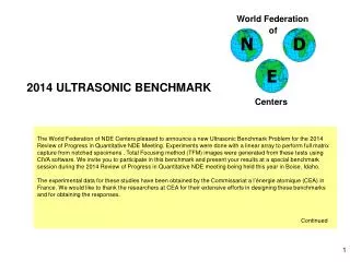
World Federation . of. N. D. E. 2014 ULTRASONIC BENCHMARK. Centers.

2014 ULTRASONIC BENCHMARK
E N D
Presentation Transcript
World Federation of N D E 2014 ULTRASONIC BENCHMARK Centers The World Federation of NDE Centers pleased to announce a new Ultrasonic Benchmark Problem for the 2014 Review of Progress in Quantitative NDE Meeting. Experiments were done with a linear array to perform full matrix capture from notched specimens . Total Focusing method (TFM) images were generated from these tests using CIVA software. We invite you to participate in this benchmark and present your results at a special benchmark session during the 2014 Review of Progress in Quantitative NDE meeting being held this year in Boise, Idaho. The experimental data for these studies have been obtained by the Commissariat a l’énergieatomique (CEA) in France. We would like to thank the researchers at CEA for their extensive efforts in designing these benchmarks and for obtaining the responses. Continued
PARTICIPATION IN THE 2014 BENCHMARK SESSION We would like to invite papers that consider the ultrasonic benchmark outlined here atthe next Annual Review of Progress in Quantitative Nondestructive Evaluation (RPQNDE) meeting. This meeting will be held July 20-25, 2014 at the Boise Center in Boise, Idaho. To present a paper at that session, please note that the deadline for submitting an abstract is Monday, April 28, 2014(mark on your abstract that it is for the benchmark session) . Also, please note that the advance registration deadline for the conference is Friday, June 20, 2014. For more details of the conference, visit the website at www.qndeprograms.org . On the following pages is a comprehensive outline of the benchmark problem being considered. You can retrieve the experimental data files at the ftp site: ftp://ftp.cea.fr/incoming/y2k01/2014_UT_benchmark/ For any questions, please e-mail Robert Sebastien at sebastien.robert@cea.fr
The 2014 UT Benchmark • Full Matrix Capture (FMC) acquisitions have been carried out to image notches in 4 specimens : • specimen 1 contains vertical notches of different heights : 2, 5 and 10 mm • specimen 2 contains identical vertical notches with different ligaments : 5 and 10 mm • specimen 3 contains identical vertical notches located at inclined backwalls : 0, 5 and 10° • specimen 4 contains identical tilted notches located at inclined backwalls : 0, 5 and 10° • The same linear phased array has been used for all the acquisitions • The used system is a MultiX system (M2M) with 128 parallel channels • FMC data are recorded in Matlab files (1 file for 1 defect) • For each acquisition, the probe has been positioned so that the angle between the probe axis and the defect direction corresponds to 45° • We will give in this document: • A description of the configurations: • specimens • defects • probe positions • A description of Matlab files • Some examples of TFM images
Description of the configurations Probe • Linear probe with 64 elementsworking at 5MHz • Whole aperture • Incident dimension : 38.3 mm • Orthogonal dimension : 10 mm • Gap between éléments: 0.1 mm • Elementwidth: 0.5 mm 38,3 mm 10 mm
Description of the configurations Specimen, defects and probe positons Specimenmaterial : carbonsteel 1020 Density: 7.8 g/cm3 cL: 5900 m/s cT: 3230 m/s Specimen1 Defect 1 10 mm 30 mm 45° 10 mm Defect 1 : side drilled hole Ø2mm Defect 1 10 mm 30 mm 45° 2 mm Defect 2 : vertical notch Defect 3 10 mm 30 mm 45° 5 mm Defect 3 : vertical notch Defect 4 10 mm 30 mm 45° 10 mm Defect 4 : vertical notch
Description of the configurations Specimen, defects and probe positons Specimenmaterial : carbonsteel 1020 Density: 7.8 g/cm3 cL: 5900 m/s cT: 3230 m/s Specimen2 10 mm ligament of 5 mm 5 mm 30 mm 10 mm 45° Defect 1 : vertical notchwith ligament 30 mm 10 mm 45° Defect 2 : vertical notchwith ligament 10 mm ligament of 10 mm 10 mm
Description of the configurations Specimen, defects and probe positons Specimenmaterial: stainlesssteel 302Density: 8.03 g/cm3 cL: 5660 m/s cT: 3120 m/s Specimen 3 Defect 1 Sidedrilledhole Ø2mm Tilt 0° 37,5 mm 45° 70 mm 10 mm 10 mm 45° Defect 2 Vertical notch , backwall orientation 0° 230 mm 37,5 mm 45° 10 mm Defect 3 Vertical notch, backwall orientation 5° 50 mm 45° 10 mm 5° Defect4 Vertical notchbackwall orientation 10° 60 mm 45° 10 mm 10°
Description of the configurations Specimen, defects and probe positons Specimenmaterial: stainlesssteel 302Density: 8.03 g/cm3 cL: 5660 m/s cT: 3120 m/s Specimen 4 Defect 1 Sidedrilledhole Ø2mm Tilt 20° 37,5 mm 45° 20° 70 mm 10 mm 45° Defect 2 Tiltednotch, backwall orientation 0° 230 mm 37,5 mm 45° 10 mm Defect 3 Tiletdnotch, backwallorientation 5° 50 mm 45° 10 mm 5° Defect4 Tiltednotch, backwall orientation 10° 60 mm 45° 10 mm 10°
Experimentaldata Full Matrix Capture data
Experimentaldata Matlab files K : matrix of the inter-element impulse responses fe : samplingfrequency (100 MHz) retard : acquisition delay (5 µs) voies : number of channels / elements (64 elements) K : 64 x 64 x 1700 Transmitters Receivers Time samples
TFM images Specimen 1 – no defect Direct mode LL
TFM images Specimen 1 – defect 1 Direct mode LL
TFM images Specimen 1 – defect2 Direct mode LL Half skip mode TTT
TFM images Specimen 1 – defect3 Direct mode LL Half skip mode TTT
TFM images Specimen 1 – defect4 Direct mode LL Half skip mode TTT
TFM images Specimen2 – defect1 Direct mode LL Half skip mode TTT Half skip mode LLT Half skip mode TLT
TFM images Specimen2 – defect2 Direct mode LL Half skip mode TTT Half skip mode LLT Half skip mode TLT
TFM images Specimen 3 – defect 1 Direct mode LL
TFM images Specimen 3 – defect2 Half skip mode LLL Half skip mode TTT Direct mode LL
TFM images Specimen 3 – defect3 Half skip mode LLL Half skip mode TTT Direct mode LL
TFM images Specimen 3 – defect 4 Half skip mode LLL Half skip mode TTT Direct mode LL
TFM images Specimen4 – defect 1 Direct mode LL
TFM images Specimen4 – defect 2 Half skip mode TTT Half skip mode LL Half skip mode LLL Half skip mode TTL
TFM images Specimen4 – defect3 Half skip mode TTT Half skip mode LL Half skip mode LLL Half skip mode TTL
TFM images Specimen4 – defect4 Half skip mode TTT Half skip mode LL Half skip mode LLL Half skip mode TTL