Download
1 / 1
10 likes | 126 Views
Implicit coupling of Lagrangian grid and solution in plasma simulation with additive Schwarz preconditioned inexact Newton. Xuefei (Rebecca) Yuan 1,4 , Stephen C. Jardin 2 , David E. Keyes 3,4 and Alice E. Koniges 1

E N D
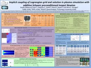
Implicit coupling of Lagrangian grid and solution in plasma simulation with additive Schwarz preconditioned inexact Newton Xuefei (Rebecca) Yuan1,4, Stephen C. Jardin2, David E. Keyes3,4 and Alice E. Koniges1 1LBNL (USA), 2PPPL (USA), 3KAUST (Saudi Arabia), 4Columbia University (USA) The work was supported by the Department of Applied Physics and Applied Mathematics of Columbia University, the Center for Simulation of RF Wave Interactions with Magnetohydrodynamics (CSWIM), and Petascale Initiative in Computational Science at NERSC . Additionally, we are grateful for the extended computer time as well as the valuable support from NERSC. This work was supported by the Director, Office of Science, Advanced Scientific Computing Research, of the U.S. Department of Energy under Contract No. DE-DC02-06ER54863. Motivation: to simulate ITER, one can estimate an additional 12 orders of magnitude are required Mathematical model: GEM magnetic reconnection By applying a mixed Lagrangian/Eulerian description of the fluid flow, 4-field extended MHD equations are transformed from the physical domain to a time-dependent curvilinear coordinate system : 1.5 orders: increased processor speed and efficiency 1.5 orders: increased concurrency 1 order: higher-order discretizations 1 order: flux-surface following gridding, less resolution required along than across field lines 4 orders: adaptive gridding, zones required refinement are < 1% of ITER volume and resolution requirements away from them are 102 less severe 3 orders: implicit solvers • the ion velocity: • the magnetic field: • the out-of-plane current density: • the Poisson bracket: • the electrical resistivity: • the collisionless ion skin depth: • the fluid viscosity: • the hyper-resistivity (or electron viscosity): • the hyper-viscosity: International Thermonuclear Experimental Reactor Nov. 2019 – First Plasma in Cadarache, France • the computational domain: , the first quadrant of the physical domain (finite difference, (anti-)symmetric fields) • boundary conditions: Dirichlet at the top, anti-symmetric in and symmetric in at other three boundaries • initial conditions: a Harris equilibrium and perturbation combination for , and other three fields are zeros Grid generation technique: the equidistribution method The logical domain: The physical domain: The transformation: Let be a two-dimensional coordinate transformation between a reference grid (a curvilinear coordinate system) and a physical grid (a Cartesian coordinate system) . Assume the transformation has the form , where is the displacement potential. A single Monge-Ampère (MA) equation leads to an adaptive grid equidistributed by the density function with the Neumann boundary condition on . The density function has the form of where, is the area of the logical domain and is provided by the user. Convergence, accuracy and complexity study • The total energy of the system is • The total energy of curvilinear solutions and Cartesian solutions approaches to at . The total energy from Asymptotic limits at Accuracy study. Take as the “exact” solution, relative errors at the final time for the curvilinear and Cartesian solutions of different problem sizes are listed. Complexity study. The number of processors (np), the problem size, the relative error, the execution time T (sec), flops F (109), memory M (107), the total number of nonlinear iterations N1, the total number of linear iterations N2, and linear iterations per nonlinear iteration N2/N1 are listed. Adaptive grids Zoom-in areas R-type adaptive grid: the current density and time-dependent coordinates The out-of-plane current density can develop large gradients and near singular behavior in the reconnection region as time evolves, requiring localized region of higher resolution. Assume is • The Cartesian solution on 256×256 is less accurate than the curvilinear solution on 64×64, so that for comparable accuracy, the curvilinear approach is 106 times more efficient. • The Cartesian solution on 256×256 is not only much less accurate than the curvilinear solution of the same size, but also with much more computational time and nonlinear, linear iterations. where , is the ratio between the biggest cell size and the smallest cell size, and is the maximum and minimum of the current density, respectively. • Thecurvilinear solutions are more accurate than the Cartesian solutions on the same problem size. The mid-plane current density vs. time: vertical axis is along the mid-plane , and the horizontal axis is time . Simulation architecture: NERSC CRAY XE6 “Hopper” Adaptive grids • 6384 nodes, 24 cores per node (153,216 total cores) • 2 twelve-core AMD ‘MagnyCours’ 2.1 GHz processors per node (NUMA) • 32 GB DDR3 1333 MHz memory per node (6000 nodes), 64 GB DDR3 1333 • MHz memory per node (384 nodes) • 1.28 Petaflop/s for the entire machine • 6 MB L3 cache shared between 6 cores on the ‘MagnyCours’ processor • 4 DDR3 1333 MHz memory channels per twelve-core ‘MagnyCours’ • processor Lagrangian and Eulerian velocities • The fluid velocity is the sum of the velocity of the grid (the Lagrangian velocity ) and the velocity of the fluid relative to the moving grid (the Eulerian velocity ): . • The temporal derivative of a scalar function defined at either a fixed spatial location or at fixed coordinates are related by the chain rule of differentiation: Compute node configuration MagnyCours processor