Download
1 / 114
1.47k likes | 2.11k Views
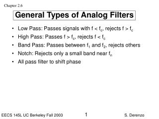
Chapter 2.6. General Types of Analog Filters. Low Pass: Passes signals with f < f c , rejects f > f c High Pass: Passes f > f c , rejects f < f c Band Pass: Passes between f 1 and f 2 , rejects others Notch: Rejects only a small band near f n All pass filter to shift phase. Chapter 2.6.

E N D
Chapter 2.6 General Types of Analog Filters • Low Pass: Passes signals with f < fc, rejects f > fc • High Pass: Passes f > fc, rejects f < fc • Band Pass: Passes between f1 and f2, rejects others • Notch: Rejects only a small band near fn • All pass filter to shift phase
Chapter 2.6 Applications of analog filters • Reduce inherent white noise (Johnson and shot) (low pass) • Reduce flicker (1/f) noise (high pass) • Baseline restoration (eliminate dc drift and instabilities- usually < 1 Hz) (high pass) • Rejecting frequencies that are more than half the sampling frequency (anti-aliasing) (low pass) • Rejecting residual carrier after demodulation or chopping (notch filter) • Reduce electromagnetic pickup (only after shielding, grounding, and differential amplification have reduced it as much as practical) (60 Hz notch filter)
Chapter 2.6 Low-Pass Filter Characteristics
Chapter 2.6 Analog Filter Characteristics • Passband: range of freq passed unaltered (gain G0) • Stopband: range of freq rejected • Corner Frequencies: drop -3 dB from passband (amplitude decreases by a factor of 0.707) • Phase Shift: between input and output waveforms- frequency dependent • Settling Time: Time for output to reach 10% of final value after step input • Order number n: Low pass amplitude drops as f–n in stopband, High pass drops as fn in stopband. (6n dB per octave, 20n dB per decade)(Butterworth and cascaded RC) • Bandwidth: Power-weightedfrequency integral
Chapter 2.6 Filter Input/Output Relations
Chapter 2.6 SimpleLow-PassFilter: StepResponse
Chapter 2.6 Simple Low-Pass Filter:Impulse Response • Impulse: T << RC • During impulse T have current I = A/R producing charge Q = IT on C • V0(t) rises linearly from 0 to AT/RC • After V1 = 0, V2(t) exponentially decreases • Ideal impulse: T 0 with AT constant
Chapter 2.6 Simple Low-Pass Filter:Frequency Response Voltage divider equation for complex impedance: factor of 2 factor of 10
Chapter 2.6 SimpleHigh-PassFilter: StepResponse
Chapter 2.6 Simple High-Pass Filter:Impulse Response • Impulse: T << RC • At start of impulse, V0 jumps up by A • During impulse T, V0 drops by AT/RC • At end of impulse, V0 jumps down by A to – AT/RC • V0 exponentially returns to zero • Ideal impulse: T 0 with AT constant ≈ Area = 0
Chapter 2.6 Simple High-Pass Filter:Frequency Response
Chapter 2.6 Square Wave Response- Simple Low and High Pass Filters f = 1/T
Chapter 2.6 Integration and Differentiationby Low and High Pass Filters • Low pass filter integrates high frequencies f >> fc, where the output falls as 1/f. • High pass filter differentiates low frequencies f << fc, where the output rises as f. • Integration of a waveform corresponds to multiplying its frequency spectrum by 1/f. (or using a LPF) • Differentiation of a waveform corresponds to multiplying its frequency spectrum by f. (or using a HPF)
Lab 6 Lab 6 - Objectives • To construct two Low-Pass, a High-Pass, and a Notch Filter using op-amp circuits • To measure their Bode amplitude and phase plots • To observe their response to a step function input • To compare measured values with the formulas for amplitude and phase vs. frequency
Lab 6 Lab 6 - Measurements to Make For: • Low-Pass, One-Pole Filter • Butterworth Low-Pass Two-Pole Filter • High-Pass, One-Pole Filter • Notch Filter Measure: • V1, V0, |G| = V0 /V1, and phase shift at 10 Hz, 100 Hz, 1 kHz, 10 kHz, 100 kHz, 1 MHz and near fc or fn • Square wave responses (sketch): • first three filters to square waves with repeat frequencies fsq = 3fc, fc, fc/3 • notch filter with fsq =fn
Lab 6 Lab 6- One-Pole, Low-Pass Filter
Lab 6 Lab 6- Butterworth Two-Pole,Low-Pass Filter
Lab 6 Lab 6- One-Pole, High-Pass Filter
Lab 6 Measurement of Phase Shift
Lab 6 Measurement of Phase Shift • Display input and output waves- trigger on input • Set vertical gain so both waves span >50% • Set vertical adjustment to center waves • Measure B1 – A1, B2 – A2, A3 – A1 A3 – A1 is period, ( A1 + A2 )/2 is time of peak of input wave, ( B1 + B2 )/2 is time of peak of output wave Phase shift P = 2π (difference in peak times)/(period)= π ( B1 + B2 – A1 – A2)/( A3 – A1 ) Note 1: Measurements made where dV/dt is large, since∆t = ∆V/(dV/dt) Note 2: Accuracy of P is insensitive to vertical adjustment in step 3
Lab 6 Alternative Measurement of Phase Shift 1 Set oscilloscope to ac coupling, set input to ground, line trigger 2 Adjust vertical shift to align trace with horizontal center line 3 Display input and output waves- trigger on input 4 Set vertical gain so both waves span >50% 5 Measure B1 – A1, A2 – A1 A2 – A1 is 1/2 periodPhase shift P = 2π (difference in first crossing times)/(period)= π ( B1 – A1)/( A2 – A1 ) Note 1: Measurements made where dV/dt is large, since∆t = ∆V/(dV/dt) Note 2: Accuracy of P is depends on vertical adjustment in step 2
Lab 6 Lab 6- Notch Filter
Lab 6 SimplifiedNotchFilterCircuit (Low Q)
Chapter 2.6 Notch Filter Characteristics • Consists of two parallel T filters • R-2C-R section is low pass with fc = 1/(4πRC) • C-R/2-C section is high pass with fc = 1/(πRC) • If components are ideal, phases cancel at fn = 1/(2πRC) • Notch depth of 30 dB typical using 5% components • To keep R > 1 kΩ and C > 100 pF, RC > 10–7 s, maximum practical notch frequency fmax < 1/(2πRC) = 1 MHz. fn – ∆f fn fn + ∆f
Chapter 2.6 Notch Filter Gain and Phase Equations
Chapter 2.6 Low-Q Notch Filter Bode Gain Plot
Chapter 2.6 Low-Q Notch Filter Phase Bode Plot
Chapter 2.6 Notch FilterResponseto TriangleWave
Chapter 2.6 High Order Filters • Butterworth Filter- flat frequency response below the corner frequency fc, but responds poorly to transients because the phase–frequency relationship is nonlinear. It is commonly used for antialiasing in circuits that sample analog waveforms because it transmits signal amplitudes faithfully. • The Bessel Filter- has a linear phase variation for frequencies below fc, and, hence, has a constant delay in this range. Since each Fourier component is shifted by the same time, the signal is transmitted without a change in shape but a constant delay is introduced. • Transitional Filter (or Paynter or “Besselworth” Filter )- has properties intermediate between those of either the Butterworth or Bessel filters. • Chebyshev Filter- maximizes the sharpness of the frequency roll-off, but introduces ripples in the passband. This filter is actually a family of filters classified by the amplitude of the ripples (in dB). Achieving the intended response requires accurate component values (typically 1 to 5%) and low-leakage capacitors. Inductors are rarely used as they are bulky and not very ideal.
Chapter 2.6 Properties of The Low PassButterworth Filter of Order n when f = fc, |G| = 0.707 (–3 dB) and = πn/4
Chapter 2.6 Bandwidth of ButterworthFilter of Order n for 1 pole, ∆f = 1.571 fc for 2 poles, ∆f = 1.111 fc for 4 poles, ∆f = 1.026 fc for 6 poles, ∆f = 1.012 fc for 8 poles, ∆f = 1.006 fc
Butterworth Filter Demo • Created a single rectangular pulse of amplitude 1 • Added 100Hz sine wave of amplitude 0.3 • Passed this signal through Butterworth low pass filters of different orders and different corner frequencies • Looking at the following series of time domain plots of the filter output, what filter parameter is changing?
Chapter 2.6 Unity-Gain Sallen-Key Filters Low Pass, two pole High Pass, two pole
Chapter 2.6 High Order Butterworth Filter Design Poles 2 4 6 8 k1 1.414 1.082 2.613 1.035 1.414 3.863 1.019 1.202 1.800 5.125 k2 0.707 0.924 0.383 0.966 0.707 0.259 0.981 0.832 0.556 0.195
Chapter 2.6 Butterworth Filter Design Example Unity-gain Sallen-Key, Butterworth high-pass four-pole filter with f0 = 10 kHz (0 = 62.83 krad/s). First Stage- From Table 2.3, k1 = 1.082 and k2 = 0.924. R1C = 1/(k10) = 1.471 10–5 R2C = 1/(k20) = 1.722 10–5 Choosing C = 1000 pF, R1 = 14.71 kΩ and R2 = 17.22 kΩ. Second Stage- k1 = 2.613 and k2 = 0.383. Choosing C = 1000 pF, R1 = 6.10 kΩ and R2 = 41.55 kΩ
Chapter 2.6 Butterworth Anti-aliasing Filter Design Design an nth order Butterworth filter with a gain > G1 for f < f1 (the passband) and a gain < G2 for f > f2 (the stopband).
Chapter 2.6 Butterworth Filter Analysis
Chapter 2.6 Frequency ratio f/fc for n-orderButterworth Low-pass filtersas a function of filter gain |G|= 0.999 0.990 0.900 0.707 0.010 0.001 0.0001 (n= 2) f/fc = 0.212 0.377 0.696 1.000 10.000 31.623 100.000 (n= 4) f/fc = 0.460 0.614 0.834 1.000 3.162 5.623 10.000 (n= 6) f/fc = 0.596 0.723 0.886 1.000 2.154 3.162 4.642 (n= 8) f/fc = 0.678 0.784 0.913 1.000 1.778 2.371 3.162 (n= 10) f/fc = 0.733 0.823 0.930 1.000 1.585 1.995 2.512 (n= 12) f/fc = 0.772 0.850 0.941 1.000 1.468 1.778 2.154
Chapter 2.6 Butterworth Filter Design Design requirements: 1 Gain > G1 for f < f1 2 Gain < G2 for f > f2 3 G = 1 at f = 0 Design procedure: 1 Tabulate fc1 (f = f1, G = G1) for a list of n values 2 Tabulate fc2 (f = f2, G = G2) for a list of n values 3 Choose smallest n value where fc1 < fc2 (i.e. the fc that satisfies the passband requirement must be lower than the fc that satisfies the stopband requirement) 4 Choose fc = (fc1 + fc2)/2 or sqrt(fc1 fc2) so both requirements are exceeded
Butterworth Filter Design Example Design a Butterworth low-pass filter that has minimum n and G > G1 = 0.9 for f < f1 = 20 kHz G < G2 = 0.01 for f > f2 = 40 kHz nf1/fcfc1 (kHz) f2/fcfc2 (kHz) 4 0.834 24.0 3.162 12.7 n too low 6 0.886 22.6 2.154 18.6 n too low 8 0.913 21.9 1.778 22.5 OK n = 8, fc = 22.2 kHz 10 0.930 21.5 1.585 25.2 n too high
Design Tips (filter choice) • Choose the Butterworth filter if the primary requirement is a flat pass band, rather than an extremely sharp frequency cutoff, or a frequency independent time delay. • Choose the Bessel filter if the primary requirement is a frequency independent time delay, however the frequency cutoff is more gradual than the Butterworth. • Choose the Transitional filter if both a flat pass band and a frequency independent time delay are important. • Choose the Chebychev filter if the primary requirement is an extremely sharp frequency cutoff, and ripples in both the time and frequency domain can be tolerated. • Choose the lowest n value that satisfies the filter requirements. A high n value increses the cost, size, and complexity of the filter. Generally, the more parts a circuit has, the higher the chance for failure.