Download
1 / 15
150 likes | 314 Views
Module 3 Decision Theory and the Normal Distribution. Prepared by Lee Revere and John Large. Learning Objectives. Students will be able to: Understand how the normal curve can be used in performing break-even analysis.

E N D
Module 3 Decision Theory and the Normal Distribution Prepared by Lee Revere and John Large M3-1
Learning Objectives Students will be able to: • Understand how the normal curve can be used in performing break-even analysis. • Compute the expected value of perfect information (EVPI) using the normal curve. • Perform marginal analysis where products have a constant marginal profit and loss. M3-2
Module Outline M3.1 Introduction M3.2 Break-Even Analysis and the Normal Distribution M3.3 EVPI and the Normal Distribution M3-3
Introduction The normal distribution can be used when there are a large number of states of nature and/or alternatives. Note: it would be impossible to develop a decision table or tree if there were 50, 100, or even more states and/or alternatives! M3-4
Break-Even Analysis and the Normal Distribution Break-even analysis, also called cost-volume analysis, answers managerial questions relating the effect of a decision to overall revenues or costs. Break-even point (units) = Fixed Costs Price/unit – Variable Costs/unit M3-5
Barclay Brothers New Product Decision The Barclay Brothers Company is a large manufacturer of adult parlor games. They are considering introducing Strategy, a new game. Their fixed cost for Strategy = $36,000 and their variable costs are $4 per game produced. They intend to sell the game for $10. What is the break-even point? Break-even point (units) = $36,000 $10 - $4 = 6,000 games M3-6
Barclay Brothers New Product Decision The Barclay Brothers expect demand to be 8,000. They believe there is a 15% chance it will be less than 5,000 and a 15% chance it will be greater than 11,000 ~ what is the probability they will lose money by not selling 6,000 games? Hint: the normal distribution can be used if the Barclay Brothers believe demand is normally distributed. M3-7
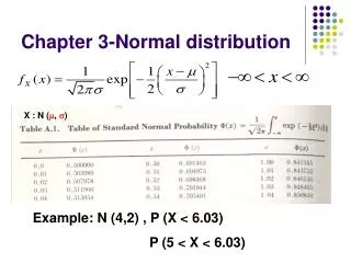
Normal Distribution for Barclay’s Demand Demand - µ Z = Mean of the Distribution, µ 15 Percent Chance Demand Exceeds 11,000 Games 15 Percent Chance Demand is Less Than 5,000 Games X 5,000 11,000 Demand (Games) µ=8,000 Use the normal table to find Z M3-8
Normal Distribution for Barclay’s Demand Look up 0.85 in the body of the normal table and find the associated Z: Z = 1.04; so 1.04 = 11,000 - 8,000 = 2,885 units What is the probability of selling less than 6,000 units???? 6,000 – 8,000 2,885 = -.69 From the table Z = .7549 so, 1 - .7549 = .2451 Or a 24.51% chance of losing $$$ ! M3-9
Barclay’s Break-Even Analysis P(loss) = P(demand < breakeven) = 0.2451 = 24.51% P(profit) = P(demand > breakeven) = 0.7549 = 75.49% Should Barclay bring its Strategy game to the market? M3-10
Expected Value of Perfect Information and the Normal Distribution The opportunity loss function describes the loss that would be suffered by making the wrong decision. The opportunity loss function can be computed by: Opportunity loss K (Break-even point - X) for X < Breakeven $0 for X > Breakeven = where K = the loss per unit when sales are below the break-even point X = sales in units. M3-11
Barclay’s Opportunity Loss Function Opportunity loss $6 (6,000 - X) for X < 6,000 games $0 for X > 6,000 games = Loss Profit Normal Distribution Loss ($) µ = 8,000 = 2,885 Slope = 6 X µ Demand (Games) Break-even point (XB) 6,000 M3-12
Expected Opportunity Loss The expected opportunity loss is the sum of the opportunity losses multiplied by the probability of that demand occurring. In the Barclay Brothers example, there are a large number of possible sales volumes (0,1,2,…5,999), so the unit normal loss integral is used. N(D) is the table value for the normal loss integral for a given value of D. M3-13
Expected Value of Perfect Information The expected value of perfect information is equivalent to the minimum EOL. EVPI = EOL = KN(D) Where EOL = expected opportunity loss K = loss per unit when sales are below the break-even point = standard deviation of the distribution µ = mean sales N(D) = the table value for the unit normal loss integral M3-14
Expected Value of Perfect Information (continued) K = $6 = 2,885 N(.69) = .1453 Therefore EOL = K N(.69) = ($6)(2885)(.1453) = $2,515.14 EVPI = $2515.14 M3-15