Postulates of Quantum Mechanics SOURCES Angela Antoniu, David Fortin, Artur Ekert, Michael Frank, Kevin Irwig , Anuj D

1. Postulates of Quantum Mechanics SOURCES Angela Antoniu, David Fortin, Artur Ekert, Michael Frank, Kevin Irwig , Anuj Dawar , Michael Nielsen Jacob Biamonte and students

2. Gates on Multi-Qubit State, a reminder

3. Example of Complex quantum system of 3 qubits – other realization of Toffoli, composed of 2-qubit gates • All gates are at most 2-qubit • Only CNOT as 2-qubit gates • It has 6 not 5 interaction gates

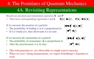
4. Linear Operators Short review • V,W: Vector spaces. • A linear operatorA from V to W is a linear function A:VW. An operator onV is an operator from V to itself. • Given bases for V and W, we can represent linear operators as matrices. • An operator A on V is Hermitian iff it is self-adjoint (A=A†). Its diagonal elements are real.

5. Eigenvalues & Eigenvectors • v is called an eigenvector of linear operator Aiff A just multiplies v by a scalar x, i.e.Av=xv • “eigen” (German) = “characteristic”. • x, the eigenvalue corresponding to eigenvector v, is just the scalar that A multiplies v by. • x is degenerate if it is shared by 2 eigenvectors that are not scalar multiples of each other. • Any Hermitian operator has all real-valued eigenvectors, which are orthogonal (for distinct eigenvalues).

6. Exam Problems • Find eigenvalues and eigenvectors of operators. • Calculate solutions for quantum arrays. • Prove that rows and columns are orthonormal. • Prove probability preservation • Prove unitarity of matrices. • Postulates of Quantum Mechanics. Examples and interpretations.

7. Unitary Transformations • A matrix (or linear operator) U is unitary iff its inverse equals its adjoint: U1 = U† • Some properties of unitary transformations (UT): • Invertible, bijective, one-to-one. • The set of row vectors is orthonormal. • The set of column vectors is orthonormal. • Unitary transformation preserves vector length: |U| = | | • Therefore also preserves total probability over all states: • UT corresponds to a change of basis, from one orthonormal basis to another. • Or, a generalized rotation of in Hilbert space Who an when invented all this stuff??

8. A great breakthrough

9. Postulates of Quantum MechanicsLecture objectives • Why are postulates important? • … they provide the connections between the physical, real, world and the quantum mechanics mathematics used to model these systems • Lecture Objectives • Description of connections • Introduce the postulates • Learn how to use them • …and when to use them

10. Physical Systems-Quantum MechanicsConnections Postulate 1 Isolated physical system   Hilbert Space Postulate 2 Evolution of a physical system   Unitary transformation Postulate 3 Measurements of a physical system   Measurement operators Postulate 4 Composite physical system   Tensor product of components

11. Postulate 1:State Space

12. Systems and Subsystems • Intuitively speaking, a physical system consists of a region of spacetime& all the entities (e.g. particles & fields) contained within it. • The universe (over all time) is a physical system • Transistors, computers, people: also physical systems. • One physical system A is a subsystem of another system B (write AB) iff A is completely contained within B. • Later, we may try to make these definitions more formal & precise. B A

13. Closed vs. Open Systems • A subsystem isclosed to the extent that no particles, information, energy, or entropy enter or leave the system. • The universe is (presumably) a closed system. • Subsystems of the universe may be almost closed • Often in physics we consider statements about closed systems. • These statements may often be perfectly true only in a perfectly closed system. • However, they will often also be approximately true in any nearly closed system (in a well-defined way)

14. Concrete vs. Abstract Systems • Usually, when reasoning about or interacting with a system, an entity (e.g. a physicist) has in mind a description of the system. • A description that contains every property of the system is an exact or concretedescription. • That system (to the entity) is a concrete system. • Other descriptions are abstractdescriptions. • The system (as considered by that entity) is an abstract system, to some degree. • We nearly always deal with abstract systems! • Based on the descriptions that are available to us.

15. States & State Spaces • A possible stateS of an abstract system A (described by a description D) is any concrete system C that is consistent with D. • I.e., it is possible that the system in question could be completely described by the description of C. • The state space of A is the set of all possible states of A. • Most of the class, the concepts we’ve discussed can be applied to eitherclassical or quantum physics • Now, let’s get to the uniquely quantum stuff…

16. An example of a state space

17. Schroedinger’s Cat and Explanation of Qubits Postulate 1 in a simple way: An isolated physical system is described by a unit vector (state vector) in a Hilbert space (state space) Cat is isolated in the box

18. Distinguishability of States • Classicalandquantum mechanicsdiffer regarding the distinguishability of states. • In classical mechanics, there is no issue: • Any two states s, t are either the same (s = t), or different (s  t), and that’s all there is to it. • In quantum mechanics (i.e.in reality): • There are pairs of states s  t that are mathematically distinct, but not 100% physically distinguishable. • Such states cannot be reliably distinguished by any number of measurements, no matter how precise. • But you can know the real state (with high probability), if you prepared the system to be in a certain state.

19. Postulate 1: State Space • Postulate 1 defines “the setting” in which Quantum Mechanics takes place. • This setting is the Hilbert space. • The Hilbert Space is an inner product space which satisfies the condition of completeness (recall math lecture few weeks ago). • Postulate1:Any isolatedphysical space is associated with a complex vector spacewith inner product called the State Space of the system. • The system is completely described by a state vector, a unit vector, pertaining to the state space. • The state space describes all possible states the system can be in. • Postulate 1 does NOT tell us either what the state space is or what the state vector is.

20. Revised Postulate 1

21. Distinguishability of States, more precisely t s  • Two state vectors s andt are (perfectly) distinguishable or orthogonal (write st) iffs†t = 0. (Their inner product is zero.) • State vectors s and t are perfectly indistinguishable or identical (write s=t) iff s†t = 1. (Their inner product is one.) • Otherwise, s and t are both non-orthogonal, and non-identical. Not perfectly distinguishable. • We say, “the amplitude of state s, given state t, is s†t”. Note: amplitudes are complex numbers.

22. State Vectors & Hilbert Space t s  • Let S be any maximal setof distinguishable possible states s, t, …of an abstract system A. • Identify the elements of S with unit-length, mutually-orthogonal (basis) vectors in an abstract complex vector space H. • The “Hilbert space” • Postulate 1: The possible states of Acan be identified with the unitvectors of H.

23. Postulate 2:Evolution

24. Postulate 2: Evolution • Evolution of an isolated system can be expressed as: where t1, t2 are moments in time and U(t1, t2) is a unitary operator. • U may vary with time. Hence, the corresponding segment of time is explicitly specified: U(t1, t2) • the process is in a sense Markovian (history doesn’t matter) and reversible, since Unitary operations preserve inner product

25. Example of evolution

26. Time Evolution • Recall the Postulate: (Closed) systems evolve (change state) over time via unitary transformations. t2 = Ut1t2 t1 • Note that since U is linear, a small-factor change in amplitude of a particular state at t1 leads to a correspondingly small change in the amplitude of the corresponding state at t2. • Chaos (sensitivity to initial conditions) requires an ensemble of initial states that are different enough to be distinguishable (in the sense we defined) • Indistinguishable initial states never beget distinguishable outcome

27. Wavefunctions • Given any set Sof system states (mutually distinguishable, or not), • A quantum state vector can also be translated to a wavefunction : S  C, giving, for each state sS, the amplitude (s) of that state. • When sis another state vector, and the real state is t, then (s) is just s†t. •  is called a wavefunction because its time evolution obeys an equation (Schrödinger’s equation) which has the form of a wave equation when S ranges over a space of positional states.

28. Schrödinger’s Wave Equation We have a system with states given by(x,t) where: • t is a global time coordinate, and • xdescribes N/3 particles (p1,…,pN/3) with masses (m1,…,mN/3) in a 3-D Euclidean space, • where each piis located at coordinates (x3i, x3i+1, x3i+2), and • where particles interact with potential energy function V(x,t), • the wavefunction (x,t) obeys the following (2nd-order, linear, partial) differential equation: Planck Constant

29. Features of the wave equation • Particles’ momentum state p is encoded implicitly by the particle’s wavelength:p=h/ • The energy of any state is given by the frequency  of rotation of the wavefunction in the complex plane: E=h. • By simulating this simple equation, one can observe basic quantum phenomena such as: • Interference fringes • Tunneling of wave packets through potential barriers

30. Heisenberg and Schroedinger views of Postulate 2 This is Heisenberg picture This is Schroedinger picture ..in this class we are interested in Heisenberg’s view…..

31. The Schrödinger Equation • The Schrödinger Equation governs the transformation of an initial input state to a final output state . It is a prescription for what we want to do to the computer. • is a time-dependent Hermitian matrix of size 2n called the Hamiltonian • is a matrix of size 2n called the evolution matrix, • Vectors of complex numbers of length 2n • Tτis the time-ordering operator

32. The Schrödinger Equation • n is the number of quantum bits (qubits) in the quantum computer • The function exp is the traditional exponential function, but some care must be taken here because the argument is a matrix. • The evolution matrix is the program for the quantum computer. Applying this program to the input state produces the output state ,which gives us a solution to the problem.

33. The Hamiltonian Matrix in Schroedinger Equation • The Hamiltonian is a matrix that tells us how the quantum computer reacts to the application of signals. • In other words, it describes how the qubits behave under the influence of a machine language consisting of varying some controllable parameters (like electric or magnetic fields). • Usually, the form of the matrix needs to be either derived by a physicist or obtained via direct measurement of the properties of the computer.

34. The Evolution Matrix in the Schrodinger Equation • While the Hamiltonian describes how the quantum computer responds to the machine language, the evolution matrix describes the effect that this has on the state of the quantum computer. • While knowing the Hamiltonian allows us to calculate the evolution matrix in a pretty straightforward way, the reverse is not true. • If we know the program, by which is meant the evolution matrix, it is not an easy problem to determine the machine language sequence that produces that program. • This is the quantum computer science version of the compiler problem.

35. Postulate 3:Quantum Measurement

36. Computational Basis – a reminder Observe that it is not required to be orthonormal, just linearly independent We recalculate to a new basis

37. Example of measurement in different bases 1/2 The second with probability zero

38. You can check from definition that inner product of |0> and |1> is zero. • Similarly the inner product of vectors from the second basis is zero. • But we can take vectors like |0> and 1/2(|0>-|1>) as a basis also, although measurement will perhaps suffer. Good base Not a base

39. A simplified Bloch Sphere to illustrate the bases and measurements You cannot add more vectors that would be orthogonal together with blue or red vectors

40. Probability and Measurement • A yes/no measurement is an interaction designed to determine whether a given system is in a certain state s. • The amplitude of state s, given the actual state t of the system determines the probability of getting a “yes” from the measurement. • Important: For a system prepared in state t, any measurement that asks “is it in state s?” will return “yes” with probability Pr[s|t] = |s†t|2 • After the measurement, the state is changed, in a way we will define later.

41. A Simple Example of distinguishable, non-distinguishable states and measurements • Suppose abstract system S has a set of only 4 distinguishable possible states, which we’ll call s0, s1, s2, and s3, with corresponding ket vectors |s0, |s1, |s2, and |s3. • Another possible state is then the vector • Which is equal to the column matrix: • If measured to see if it is in state s0,we have a 50% chance of getting a “yes”.

42. Observables • Hermitian operator A on V is called an observable if there is an orthonormal (all unit-length, and mutually orthogonal) subset of its eigenvectors that forms a basis of V. There can be measurements that are not observables Observe that the eigenvectors must be orthonormal

43. Observables • Postulate 3: • Every measurable physical property of a system is described by a corresponding operator A. • Measurement outcomes correspond to eigenvalues. • Postulate 3a: • The probability of an outcome is given by the squared absolute amplitude of the corresponding eigenvector(s), given the state.

44. Density Operators • For a given state |, the probabilities of all the basis states si are determined by an Hermitian operator or matrix  (the density matrix): • The diagonal elementsi,iare the probabilities of the basis states. • The off-diagonal elements are “coherences”. • The density matrix describes the state exactly.

45. Towards QM Postulate 3 on measurement and general formulas Pm| p(m) A measurement is described by an Hermitian operator (observable) M = m Pm • Pm is the projector onto the eigenspace of M with eigenvalue m • After the measurement the state will be with probability p(m) = |Pm|. • e.g. measurement of a qubit in the computational basis • measuring | = |0 + |1 gives: • |0 with probability |00| = |0||2 = ||2 • |1 with probability |11| = |1||2 = ||2 eigenvalue  m

46. Duals and Inner Products are used in measurements <| This is inner product not tensor product! ( ) Remember this is a number We prove from general properties of operators

47. Duals as Row Vectors To do bra from ket you need transpose and conjugate to make a row vector of conjugates.

48. General Measurement To prove it it is sufficient to substitute the old base and calculate, as shown

49. Illustration of some formalisms used, you can calculate measurements from there q State Vector Density State

50. Postulate 3, rough form This is calculate as in previous slide