
Lexical Analysis
E N D
Presentation Transcript
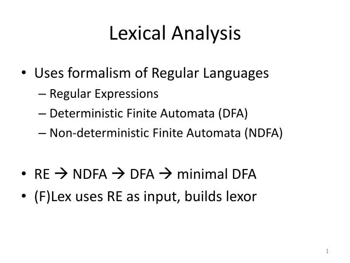
Lexical Analysis • Uses formalism of Regular Languages • Regular Expressions • Deterministic Finite Automata (DFA) • Non-deterministic Finite Automata (NDFA) • RE NDFA DFA minimal DFA • (F)Lex uses RE as input, builds lexor
Regular Expressions • Regular expression (over S) • • e • a where aS • r+r’ • r r’ • r* • where r,r’ regular (over S) • Notational shorthand: • r0 = e, ri = rri-1 • r+ = rr*
DFAs: Formal Definition DFA M = (Q, S, d, q0, F) Q = states finite set S = alphabet finite set d = transition function function in Q S Q q0 = initial/starting state q0 Q F = final states F Q
a b …aa …ab b a a a e b a b a b b …ba …bb a a b b DFAs: Example strings over {a,b} with next-to-last symbol = a
Nondeterministic Finite Automata “Nondeterminism” implies having a choice. Multiple possible transitions from a state on a symbol. d(q,a) is a set of states d : Q S Pow(Q) Can be empty, so no need for error/nonsense state. Acceptance: exist path to a final state? I.e., try all choices. Also allow transitions on no input: d : Q (S {e}) Pow(Q)
S a …a …aS … S Loop until we “guess” which is the next-to-last a. NFAs: Example strings over {a,b} with next-to-last symbol = a
CFGs: Formal Definition G = (V, S, P, S) V = variables, a finite set S = alphabet or terminals a finite set P = productions, a finite set S = start variable, SV Productions’ form, where AV, a(VS)*: • A a
CFGs: Derivations Derivations in one step: bAgGbag Aa P xS*, a,b,g(VS)* Can choose any variable for use for derivation step. Derivations in zero-or-more steps: G* is the reflexive and transitive closure of G . Language of a grammar: L(G) = {xS* | S G* x}
S A B Root label = start node. A A b B Each interior label = variable. a a b Each parent/child relation = derivation step. Each leaf label = terminal or e. All leaf labels together = derived string = yield. Parse Trees S A | A B A e | a | A b | A A B b | bc | B c | b B • Sample derivations: • S AB AAB aAB aaB aabB aabb • S AB AbB Abb AAbb Aabbaabb These two derivations use same productions, but in different orders.
S A B A A b B a a b Left- & Rightmost Derivations S A | A B A e | a | A b | A A B b | bc | B c | b B • Sample derivations: • S AB AAB aAB aaB aabB aabb • S AB AbB Abb AAbb Aabbaabb • These two derivations are special. • 1st derivation is leftmost. • Always picks leftmost variable. • 2nd derivation is rightmost. • Always picks rightmost variable.
Disambiguation Example Exp n | Exp + Exp | Exp Exp What is an equivalent unambiguous grammar? Exp Term | Term + Exp Term n | n Term Uses • operator precedence • left-associativity
Parsing Designations • Major parsing algorithm classes are LL and LR • The first letter indicates what order the input is read – L means left to right • Second letter is direction in the “parsing tree” the derivation goes, L = top down, R = bottom up • K of LL(k) or LR(k) is number of symbols lookahead in input during parsing • Power of parsing techniques • LL(k) < LR(k) • LL(n) < LL(n+1), LR(n) < LR(n+1) • Choice of LL or LR largely religious
Items and Itemsets • An itemset is merely a set of items • In LR parsing terminology an item • Looks like a production with a ‘.’ in it • The ‘.’ indicates how far the parse has gone in recognizing a string that matches this production • e.g. A -> aAb.BcC suggests that we’ve “seen” input that could replace aAb. If, by following the rules we get A -> aAbBcC. we can reduce by A -> aAbBcC
Building LR(0) Itemsets • Start with an augmented grammar; if S is the grammar start symbol add S’ -> S • The first set of items includes the closure of S’ -> S • Itemset construction requires two functions • Closure • Goto
Closure of LR(0) Itemset If J is a set of items for Grammar G, then closure(J) is the set of items constructed from G by two rules 1) Each item in J is added to closure(J) 2) If A α.Bβ is in closure(J) and B φ is a production, add B .φ to closure(J)
Closure Example Grammar: A aBC A aA B bB B bC C cC C λ Closure(J) A a.BC A-> a.A A .aBC A .aA B .bB B .bC J A a.BC A a.A
GoTo Goto(J,X) where J is a set of items and X is a grammar symbol – either terminal or non-terminal is defined to be closure of A αX.β for A α.Xβ in J So, in English, Goto(J,X) is the closure of all items in J which have a ‘.’ immediately preceding X
Set of Items Construction Procedure items(G’) Begin C = {closure({[S’ .S]})} repeat for each set of items J in C and each grammar symbol X such that GoTo(J,X) is not empty and not in C do add GoTo(J,X) to C until no more sets of items can be added to C
Build LR(0) Itemsets for: • {S (S), S λ} • {S (S), S SS, S λ}
Building LR(0) Table from Itemsets • One row for each Itemset • One column for each terminal or non-terminal symbol, and one for $ • Table [J][X] is: • Rn if J includes A rhs., A rhs is rule number n, and X is a terminal • Sn if Goto(J,X) is itemset n
LR(0) Parse Table for: • {S (S), S λ} • {S (S), S SS, S λ}
Building SLR Table from Itemsets • One row for each Itemset • One column for each terminal or non-terminal symbol, and one for $ • Table [J][X] is: • Rn if J includes A rhs., A rhs is rule number n, X is a terminal, AND X is in Follow(A) • Sn if Goto(J,X) is itemset n
LR(0) and LR(1) Items • LR(0) item “is” a production with a ‘.’ in it. • LR(1) item has a “kernel” that looks like LR(0), but also has a “lookahead” – e.g. A α.Xβ, {terminals} A α.Xβ, a/b/c ≠ A α.Xβ, a/b/d
Closure of LR(1) Itemset If J is a set of LR(1) items for Grammar G, then closure(J) includes 1) Each LR(1) item in J 2) If A α.Bβ, a in closure(J) and B φ is a production, add B .φ, First(β,a) to closure(J)
LR(1) Itemset Construction Procedure items(G’) Begin C = {closure({[S’ .S, $]})} repeat for each set of items J in C and each grammar symbol X such that GoTo(J,X) is not empty and not in C do add GoTo(J,X) to C until no more sets of items can be added to C
Build LR(1) Itemsets for: • {S (S), S SS, S λ}
{S CC, C cC, C d} Is this grammar • LR(0)? • SLR? • LR(1)? How can we tell?
LR(1) Table from LR(1) Itemsets • One row for each Itemset • One column for each terminal or non-terminal symbol, and one for $ • Table [J][X] is: • Rn if J includes A rhs., a; A rhs is rule number n; X = a • Sn if Goto(J,X) in LR(1) itemset n
LALR(1) Parsing • LookAhead LR (1) • Start with LR(1) items • LALR(1) items --- combine LR(1) items with same kernel, different lookahead sets • Build table just as LR(1) table but use LALR(1) items • Same number of states (row) as LR(0)
Code Generation • Pick three registers to be used throughout • Assuming stmt of form dest = s1 op s2 • Generate code by: • Load source 1 into r5 • Load source 2 into r6 • R7 = r5 op r6 • Store r7 into destination
Three-Address Codesection 6.2.1 (new), pp 467 (old) • Assembler for generic computer • Types of statements 3-address (Dragon) • Assignment statement x = y op z • Unconditional jump br label • Conditional jump if( cond ) goto label • Parameter x • Call statement call f
Example “Source” a = ((c-1) * b) + (-c * b)
Example 3-Address t1 = c - 1 t2 = b * t1 t3 = -c t4 = t3 * b t5 = t2 + t4 a = t5
Three-Address Implementation(Quadruples, sec 6.2.2; pp 470-2)
Three-Address Implementation • N-tuples (my choice – and yours ??) • Lhs = oper(op1, op2, …, opn) • Lhs = call(func, arg1, arg2, … argn) • If condOper(op1, op2, Label) • br Label
Three-Address Code • 3-address operands • Variable • Constant • Array • Pointer
Variable Storage Memory Locations (Logical) Stack Heap Program Code Register Variable Classes Automatic (locals) Parameters Globals
Variable Types • Scalars • Arrays • Structs • Unions • Objects ?
Row Major Array Storage char A[20][15][10];
Column Major Array Storage char A[20][15][10];
OR (Row Major) char A[20][15][10];
Array Declaration Algorithm Dimension Node { int min; int max; int size; }
Declaration Algorithm (2) • Doubly linked list of dimension nodes • Pass 1 – while parsing • Build linked list from left to right • Insert min, max • Size = size of an element (e.g. 4 for int) • Append node to end of list • min = max = size = 1
Declaration Algorithm (3)Pass 2 • Traverse list from tail to head • For each node, n, going “right” to “left” • Factor = n.max – n.min + 1 • For each node, m, right to left starting with n • m.size = m.size * factor • For each node, n, going right to left • max = N->left->max; min = N->left->min • Save size of first node as size of entire array • Delete first element of list • Set tail->size = size of an element (e.g. 4 for int)
Array Declaration (Row Major) int weight[2000..2005][1..12][1..31]; list of “dimension” nodes int min, max, size size of element of this dimension 1448 124 4
Array Offset (Row Major) Traverse list summing (max-min) * size int weight[2000..2005][1..12][1..31]; x = weight [2002][5][31] (2002-2000) * 1448 + (5-1) * 124 + (31-1) * 4 1448 124 4
Array Offset (Row Major) Traverse list summing (max-min) * size int weight[2000..2005][1..12][1..31]; x = weight [i][j][k] (i - 2000) * 1448 + (j-1) * 124 + (k-1) * 4 1448 124 4
Your Turn • Assume • int A[10][20][30]; • Row major order • “Show” A’s dimension list • Show hypothetical 3-addr code for • X = A[2][3][4] ; • A[3][4][5] = 9
My “Assembly” code X = A[2][3][4]; T1 = 2 * 2400 T2 = 3 * 120 T3 = T1 + T2 T4 = 4 * 4 T5 = T3 + T4 T6 = T5 + 64 # 64 is A’s offset %eax = T5 %eax = %ebp + %eax %eax = 0(%eax) 16(%ebp) = %eax # 16 is X’s offset