In Situ Measurements of Surface Gravity Waves in Typhoon Conditions

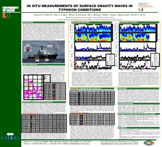
1. In Situ Measurements of Surface Gravity Waves in Typhoon Conditions Clarence O. Collins III1, Hans C. Graber1, William M. Drennan1, Neil J. Williams1, Rafael J. Ramos1, Bjoern Lund1, and Eric J. Terrill2 1)Rosenstiel School of Marine and Atmospheric Science (RSMAS), University of Miami 2) Scripps Institution of Oceanography, University of California, San Diego, 9500 Gilman Drive, La Jolla CA, 92093 a) a) Dianmu Fanapi Malakas Megi Chaba Dianmu Fanapi Malakas Megi Chaba b) b) c) c) MWB WaMoS d) d) EASI ASIS e) e) Photo Credit: Dr. Hans C. Graber The figure above includes EASI spectral density evolution, EASI directional distribution evolution, and the time series of bulk parameters from all sensors involved in the comparison. The NZ and SZ are on the left and right, respectively. Panel a) This shows the evolution of the frequency spectrum. The spectral density, represented by color, is on a natural log scale to emphasize the high frequency end of the spectra. Panel b) This is the evolution of the directional distribution. First each frequency spectra is normalized by its maximum spectral energy. Then the direction distributions were calculated using the Longuet-Higgins weighted Fourier expansion method. This method is known to artificially increase the directional spread. The EASI buoy can only measure the 2 lowest directional moments rendering the plot qualitative in essence, but it clearly compliments information from the WD [panel e)]. Panel c) This is Hs. In the NZ the highest wave heights are associated with the passage of Typhoon Chaba around year day 300, whereas in the SZ the highest wave heights are associated with Typhoon Megi around year day 290. Panel d) This is peak period. The isolated points are probably due to low fidelity during low sea-states. These points are to be investigated further in the future. The longest waves are associated with the Megi and Chaba, but the period also becomes quite long around year day 270. This is most likely associated with swell which emanated from Typhoon Malakas around 2000km to the North-East. The wave height is slightly higher and more peaked in the NZ during this time indicating dispersion as the waves traveled south. Panel e) This is WD. There is good agreement and similar scatter among the buoys. The WaMoS exhibits less scatter than the buoys, and has a higher directional resolution in general. Future work will compare directional spread as well. analysis shows similar results with comparisons made within smaller radii (i.e. 25km, 50km). The mean distance to the mobile platforms is actually much less than 100km. The criterion is slightly relaxed for measurements made during a particular pass of Jason-1. This work would not have been possible without the technical support of Mike Rebozo (RSMAS). Thanks to Henry Potter (RSMAS), Michele Gierach (RSMAS), Ian Brooks (Leeds), Dominic Salisbury (Leeds), Sara Norris (Leeds), Sharein E-Tourky (RSMAS) and Anibal Herrera (RSMAS) who were cruise participants. Thanks to Mike Ohmart and Avery Snyder (UW-APL) for help with ASIS recoveries. Thanks to the captains and crew of the R/V Roger Revelle, and the WHOI mooring operations team. Funding provided by the U.S. Office of Naval research. Peak period, although a common parameter, is not a vary stable measure of period. This lack of stability is reflected in the low correlation coefficients and high standard differences. There are also isolated points (suspected to spurious) which throw off the comparative results. Even so, it is estimated that most of variability can be explained by the inherent sampling variability of the parameter. Future work will explore more stable period parameters. WAVE DIRECTION AT THE PEAK The table above shows the number of points, the fit parameters for a maximum likelihood regression, a directional association measure, directional bias, and directional standard difference. The direction at the peak is also an unstable parameter. Directionally multi-modal seas (which the buoys cannot resolve) with similar energies in each mode are a possibility. The multi-modality causes the peak direction to jump back and forth between peaks. The jumping causes comparisons to be poor and muddles the interpretation of results. It is suspected that multi-modal seas occur throughout the experiment, but this is speculation until it can be further investigated with the superior directional resolution of the WaMoS. Considering this, the wave directions compare surprisingly well with very high associations. Future work will include comparisons of more stable measures of mean direction, comparison of directional spread, investigation of higher-order methods to calculate directional spectra from EASI, and investigation of directional modality. The tables show the # of points, fit parameters for a maximum likelihood regression, the correlation coefficient, bias, standard difference, estimated coefficient of variance, and the percentage of points that fall within a 90% confidence interval with and without bias. The comparisons are very good in general with most R values ≥ .90. The notable exception is EASI S vs MWB 43. The comparison was during Tropical Cyclone Diamnu. It is suspected that there was unusually strong spatial variability in Hs at the time, and is a matter for future investigation. Clarence O. Collins III, RSMAS-AMP, 4600 Rickenbacker Cswy, Miami FL 33149 USAPhone: +1 305 421 4282, Fax: +1 305 421 4701, E-Mail: tcollins@rsmas.miami.edu This work has been funded by the U.S. Office ofNaval Research under grant N00014-08-1-0581