Download

1 / 74
740 likes | 1.03k Views
Macroeconomic Consequences of the Demographic Transition. Ronald Lee UC Berkeley July 9, 2008 Talk prepared for Rand Summer Institute Research supported by NIA R37 AG025247 Thanks to Andy mason and NTA country teams . Plan. Demographic transition Dependency ratios and support ratios

E N D
Macroeconomic Consequences of the Demographic Transition Ronald Lee UC Berkeley July 9, 2008 Talk prepared for Rand Summer Institute Research supported by NIA R37 AG025247 Thanks to Andy mason and NTA country teams Data from
Plan • Demographic transition • Dependency ratios and support ratios • Savings rates and capital intensification • Human capital Data from
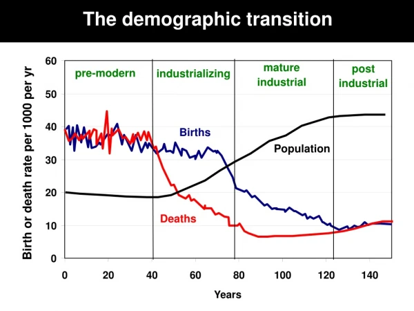
I. The Demographic Transition • A classic illustration: The transition in India, 1890-2100. • Mixture of historical estimates, UN projections, and simulation based on fitted variations with time. Data from
Pre fertility decline; child dependency ratio rises During fertility decline, child dependency ratio declines Population aging: old age dep ratio rises Data from
The total dep ratio rises, falls, then rises again, ending up where it started. The changes in the total dependency ratio are transitory. Data from
But there is a big permanent change: At start, many children and few elderly. At end, few children and Many elderly. Data from
Comments on simulation • Assumed TFR stabilized at 2.1; but often has declined below replacement. • Assumed e0 stopped rising at 80, but many countries already above this. • Some countries experienced important baby booms and busts which distort this classic shape. • Many countries now have declining populations and declining working age pops. Data from
II. The economic life cycle: • Age profiles of consumption and labor income • Use estimates from the National Transfer Accounts project, or NTA. • Consumption patterns are quite similar for Third World countries in Asia and Latin America. • Consumption in Industrial populations looks different. Data from
Includes self employment, wages,unpaid family labor, & fringe benefits. Averages 0’s and both male and female. Includes both private expends and in-kind public transfers (health, education, long term care) Data from An-Chi Tung
Flat cons age profile in adult years reflects extended family sharing. Quite different than most industrial nations. Data from An-Chi Tung
Large deficits at young and old ages. Data from An-Chi Tung
Reallocations from surplus to deficit ages required. Data from An-Chi Tung
Other income comes from assets, foreign loans, and remittances from abroad—its not all labor income. Data from An-Chi Tung
Asset income is partic Impt for old age Data from An-Chi Tung
Components of US Consumption, 2003 Unlike Taiwan and other Third World, in US cons rises strongly with age. True in other industrial too. Later I will measure HK investment As sum of pub and priv spending on hlth and educ as shown here. Data from
Levels of age profiles change fast with economic development. • Shapes of age profiles change slowly, • Are broadly similar across countries at very different levels of development.
III. Dependency and Support • Concern about pop aging is mostly about old age dependency. • Sharpest concerns for age-sensitive public sector programs • pensions • health care • Long term care • But should place these in broader context • Full range of public programs • Private consumption • Use shape of estimated profile I just showed.
Support Ratios • Effective labor is weighted sum of pop using labor income age profile. • Effective consumers is similar. • Ratio of effective labor to effective consumers is the “Support Ratio”. • Other things equal, consumption per effective consumer is proportional to the support ratio.
Population aging First Dividend
Proportionate Changes in the Support Ratio from 2007 to 2050 for Selected MDC and LDC
Not written in stone. Many policy possibilities: • Change the age profile of labor income • Later retirement • Earlier entry into labor force • Higher female labor force participation • Reform seniority system • Change the age profile of consumption • In many industrial nations, the elderly consume much more than younger adults. • Makes population aging more costly • Role of public transfer policy: pensions, health care, long term care • Change the demographic trends: immig, fert
IV. Further on Interage Flows of Income • Comparison of Japan and Indonesia
Per capita consumption and labor income by age for Indonesia and Japan • Differences in consumption • Education in Japan • Rising consumption in old age in Japan Indonesia, 2002 Japan, 2004 Data from Maliki (Indonesia) and H. Ogawa (Japan)
Green arrows show transfers from surplus of prime working years. • Red arrows show asset income consumed by elderly out of earlier savings. Data from Maliki (Indonesia) and H. Ogawa (Japan)
Population weighted average age Ac=30 Ayl=39 Indonesia, 2002 • In Indonesia, average unit of income is earned at 39 and consumed at 30 • Travels 9 years down the age scale. • In Japan, it is earned and consumed at nearly the same age. Ac=45 Ayl=45 Japan, 2004 Data from Maliki (Indonesia) and H. Ogawa (Japan)
Average Consumption-Earning Gap by Average Age of Population 13 yrs Data from NTA Country Teams
How much of the difference in age gaps is due to the shapes of the age profiles? Data from NTA Country Teams
Average Age of Labor Income and Consumption with Population Held Constant (stationary, e0=75) Data from NTA Country Teams
Average Age of Labor Income and Consumption with Population Age Distr. Constant (stationary, e0=75) High cons (health care) and work when old. Low age of cons due to heavy spending on education. Low age of cons due to heavy spending on education. Low age of cons due to heavy spending on education. Low age of cons due to heavy spending on education. Low age of cons due to heavy spending on education. Low age of cons due to heavy spending on education. Generous old age support. Very young Ayl due to early start, early retirement. Data from NTA Country Teams
Average Age of Labor Income and Consumption with Population Held Constant (stationary, e0=75) Difference in average ages is the distance above (-) or below (+) the diagonal. Data from NTA Country Teams
Average Age of Labor Income and Consumption with Population Held Constant (stationary, e0=75) Indonesia -3.3 yrs Austria +2.2 yrs Data from NTA Country Teams
total range in age gap was 13 years • range due to differences in profiles is 5.5 years. • So both population age distribution and shapes of age profiles help determine gap.
V. Wealth and the age gap: the golden rule case • Demographic and economic steady state • Saving and capital such as to maximize per capita consumption. • r=n+g
Now suppose babies had to go into debt to feed themselves…. • At the start of life, c(x)>yl(x); dependency. • Suppose we keep a notional account of debt and credit over the life cycle, discounted to age 0. • Credit gained (or lost) at age x is: e-rx l(x) [yl(x)-c(x)] wherer is interest rate, l(x) is survival from 0 to age x. • Cumulated up to age x, we get W(x):
The average wealth per capita in the population may be pos or neg • Now find the average level of per capita in the whole population, call it W • W = pop(x)*W(x)/totpop
The Willis result W = c(Ac – Ay) , where c = per capita cons • If Ac>Ay then indivs need to hold onto some output for later consumption, so wealth, W, is on average positive in the population. • If Ac<Ay then indivs consume before they produce, and must go into debt on average, so W is negative. • Alternatively: W/c = Ac – Ayl • So wealth relative to consumption is roughly proportional to Ac - Ayl
Given comparative analysis of Ac-Ayl, suggests that demand for wealth rises over the demographic transition. • Why? • Older people hold more wealth; in old population, there are more of them. • Longer life means workers need to accumulate more wealth for longer old age. • Lower fertility means adults consume more and need to save more to maintain in old age.
VI. The role of intergenerational transfers • We just considered the wealth needed to achieve consumption targets. • Wealth can be held in two forms: • Transfer wealth (expected future transfers received minus expected future transfers made) • Assets or Capital
NTA data on shares of old age support from different sources • Asset income (land, equities, interest, etc.) • Family transfers (not including bequests at death) • Public transfers (Pay As You Go pensions, health care, and long term care) • Triangle graph shows shares, not levels, so must add to 100%. • Bequests not included; just old age cons.
Familial transfers equally important in Thailand, Korea, and Taiwan (36-40%). Net public transfers to elderly are zero in Thailand; about 25% in Taiwan and Korea. Net familial transfers near zero in US, CR, and J. Large public transfers in CR and J Diagram from Andy Mason
Public transfers: Thailand none, Japan and Costa Rica around 70% US, Korea, Taiwan, middling Diagram from Andy Mason
Reliance on assets : Japan, Taiwan, C.R. are low; Thailand high; US middling Diagram from Andy Mason
VII. Demographic Transition and Capital Accumulation • Changing dependency gets most attention for ec dev and pop aging. • Changes in capital accumulation may be more important.
Calculating the demand for wealth and capital over the demographic transition • Based on different theoretical models, approaches. • Model with Social Planner maximizing discounted social welfare function with full foresight. • Model with individuals saving and consuming over their life cycles to maximize their life time utility.