Download
1 / 23
230 likes | 387 Views
High Speed Imaging of Edge Turbulence in NSTX. S.J. Zweben, R. Maqueda 1 , D.P. Stotler, A. Keesee 2 , J. Boedo 3 , C. Bush 4 , S. Kaye, B. LeBlanc, J. Lowrance 5 , V. Mastrocola 5 , R. Maingi 4 , N. Nishino 6 , G. Renda 5 , D. Swain 4 , J. Wilgen 4 and the NSTX Team

E N D
High Speed Imaging of Edge Turbulence in NSTX S.J. Zweben, R. Maqueda1, D.P. Stotler, A. Keesee2, J. Boedo3, C. Bush4, S. Kaye, B. LeBlanc, J. Lowrance5, V. Mastrocola5, R. Maingi4, N. Nishino6, G. Renda5, D. Swain4, J. Wilgen4 and the NSTX Team Princeton Plasma Physics Laboratory, Princeton, NJ 1 Los Alamos National Lab, Los Alamos, NM 2 West Virginia University, Morgantown, WV 3 UCSD, San Diego, CA 4 Oak Ridge National Laboratory, Oak Ridge, TN 5 Princeton Scientific Instruments Inc, Monmouth Junction, NJ 6 Hiroshima University, Hiroshima, Japan TTF Meeting, Madison Apr. 3, 2003
Outline • Goals • Fisheye view of NSTX • Gas puff imaging diagnostic • GPI image and time series analysis • Summary • Plans
Goals • Understand edge turbulence by comparing turbulence measurements with theory + simulation • Explain and predict H-mode threshold and pedestal • Explain and predict transport through SOL to wall • Explain and predict transport of impurities into plasma • Explain and predict density limit ?
Fisheye View of NSTX LANL camera, 10 µsec/frame at 1000 frames/sec no filter (mainly D light) Magnetic structure of edge plasma
Gas Puff Imaging Diagnostic • Look at He1(578.6 nm) from gas puff I none f(ne,Te) • View along B field line to see 2-D structure B GPI view 16x32 cm
out 200 sep. DEGAS HeI n(Heo) 100 GPI HeI 0 ne/1011 cm-3 Te(eV) RMP(cm) Typical GPI Image • Use typically 10 µsec exposure time (tac ≈ 40 µsec) • Average HeI light intensity peaked near separatrix PSI camera frame 80 x 160 pixels
GPI Diagnostic Interpretation • • HeI light emission “I” visible where 5 eV < Te < 50 eV • • I neaTeb,wherea ≈0.5and b ≈0.7near center of cloud, • with 0.4 < a < 1 and 0 < b < 2over most of cloud • • Space-time structure of I similar to nea, but dI/I ≈ adne/ne • • Fluctuation spectra of I similar to probe and reflectometer • • Fluctuation level of I consistent with TS data ( ≈10-60%) • GPI light gives approximate structure of edge turbulence
High Speed Imaging of NSTX Edge CCD camera with 100,000 frames/sec at 10 µsec/frame for 28 frames/shot localized structures can move outward at ≈ 105 cm/sec
Profiles from Typical GPI Images • HeI profiles narrow from OH to L-mode to H-mode • dI/I and Lpol derived from 28 images for each shot A(k) L(cm) kpol(cm-1) dI/I
Poloidal Correlation Length and k-spectra • Lpol ≈ 4 cm or kpol rs ≈0.2(similar to other experiments) • dI/I lower in H-mode than L-mode (with much variation)
Time (sec) Time Series of GPI Light Flucutuaions • HeI digitized over 1.5 cm diam. chords through images • Relative fluctuation level larger as R increases (≈ images)
Statistical Analysis of Typical Chords • Autocorrelation times typically 40 ± 20 µsec • Frequency spectra broad over ≈ 0.1 - 100 kHz Autocorrelation function Frequency spectrum Probability distribution function
L-H and H-L Transitions • L -> H in ≈ 100 µsec with obvious precursor • H -> L in 30 µsec with outward radial pulse 1 ms 100 µs
Slow Imaging of H-L Transition • Taken with 10 µsec exposures at 1000 frames/sec • For this display, outward direction toward lower right H-L (#105710) L-H-L (#105564)
Motion of Coherent Structures • Track high intensity “blobs” over 28 frames of movies • Broad distribution of velocities and intensities
Summary of Results So Far • Images consistent with previous measurements - large fluctuation level in edge - broad frequency and k-spectrum - approx. isotropic structure B • Coherent structures seem to move through edge - “blob- like” look similar to DIII-D IPOs - “wave-like” look similar to EDA, QCM • H-mode generally more quiescent than L-mode - considerable variation in behavior - transitions can happen very fast
Plans for Comparison with Theory Using DEGAS-2 or related atomic physics models: • Compare GPI with BOUT simulations for H- and L-mode (Xu and Nevins) • Compare motion of GPI “blobs” with blob model (D’Ippolito and Myra) • Compare with other simulations…
Plans for Additional Measurements • Capture H-mode transition with high speed camera • Get better data on zonal flows in images and chords • Examine turbulence nearer density limit • Look during RF heating, e.g. co- vs. ctr. current drive • Make systematic scans of q(a), rotation, Zeff, etc. • Make quantitative comparisons with other diagnostics
a HeI (rel.) Alpha b RMP(cm) Fluctuation level (rel.) Correlation length (rel.) Alpha Alpha (b) (a) (3) (1) Amplitude (rel.) (2) Wavenumber (rel.) (c) (3) (d) (2) (1)
#105637 dI/I (rel.) LCFS RMP(cm)
x probe before puff • probe during puff o GPI during puff Power (rel.) Frequency (kHz)
1 0.1 0.01 0.001 0.0001 10-5 x reflectometer before puff • reflectometer during puff o GPI during puff Power (rel.) Frequency (kHz)
n/n T/T n/n T/T n/n T/T RMP(cm) RMP(cm)