Download
1 / 38
380 likes | 582 Views
Understand various point interpolation methods in GIS analysis, including linear and non-linear techniques, global vs local strategies, trend surfaces, splines, Inverse Distance Weighted method, and Kriging. Learn how to estimate values at unsampled locations.

E N D
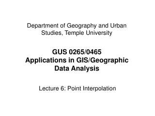
Department of Geography and Urban Studies, Temple UniversityGUS 0265/0465Applications in GIS/Geographic Data Analysis Lecture 6: Point Interpolation
Interpolating a Surface From Sampled Point Data • Assumes a continuous surface that is sampled • Interpolation • estimating the attribute values of locations that are within the range of available data using known data values • Extrapolation • estimating the attribute values of locations outside the range of available data using known data values
Interpolation Estimating a point here: interpolation Sample data
Extrapolation Sample data Estimating a point here: extrapolation
Linear Interpolation If A = 8 feet and B = 4 feet then C = (8 + 4) / 2 = 6 feet Sample elevation data A C B Elevation profile
Non-Linear Interpolation Sample elevation data Often results in a more realistic interpolation but estimating missing data values is more complex A C B Elevation profile
Exact Interpolation Sample elevation data Interpolated surface passes through the original data points Elevation profile
Inexact Interpolation Sample elevation data Interpolated surface does not pass through all of the original data points Elevation profile
Global Interpolation Uses all known sample points to estimate a value at an unsampled location Sample data
Local Interpolation Uses a neighborhood of sample points to estimate a value at an unsampled location Sample data Uses a local neighborhood to estimate value, i.e. closest n number of points, or within a given search radius
Trend Surface Global method Inexact Can be linear or non-linear Multiple regression (e.g. predicting a z elevation value [dependent variable] with x and y location values [independent variables])
1st Order Trend Surface In one dimension: z varies as a linear function of x z z = b0 + b1x + e x
1st Order Trend Surface In two dimensions: z varies as a linear function of x and y z y z = b0 + b1x + b2y + e x
2nd Order Trend Surface In one dimension: z varies as a non-linear function of x z = b0 + b1x + b2x2 + e z x
Splines Local method Can be exact or inexact Non-linear Derived from the use of flexible rulers for drafting Fits a piece-wise polynomial function to a neighborhood of sample points Typically produces a smooth surface
Thin Plate Spline Minimizes curvature while ensuring interpolated surface passes through the sampled points Can adjust the tension of the spline to address ‘overshoot’ problem where estimates are too high due to the modeled curvature of the surface
Splines In one dimension In two dimensions z y y x x
Inverse Distance Weighted (IDW) Local method Exact Can be linear or non-linear The weight (influence) of a sampled data value is inversely proportional to its distance from the estimated value
Inverse Distance Weighted (IDW) • In English: • Find the neighboring sample points of the target location (i.e. through n nearest neighbors or a search radius) • Find the distance from each sample point to the target location • Weight each sample point according to the inverse of its distance from the target location taken to the r exponent • Average the weighted attribute values of the sample points and assign the resulting value to the target location
Inverse Distance Weighted (IDW): Example 100 IDW: Closest 3 neighbors, r = 2 4 3 160 2 200
Inverse Distance Weighted (IDW): Example Weights A BC 1 / (42) = .0625 1 / (32) = .1111 1 / (22) = .2500 A = 100 4 B = 160 3 2 C = 200
Inverse Distance Weighted (IDW): Example Weights A BC 1 / (42) = .0625 1 / (32) = .1111 1 / (22) = .2500 The weight = inverse of the distance squared A = 100 4 B = 160 3 2 C = 200
Inverse Distance Weighted (IDW): Example Weights Weights * Value A BC 1 / (42) = .0625 1 / (32) = .1111 1 / (22) = .2500 .0625 * 100 = 6.25 .1111 * 160 = 17.76 .2500 * 200 = 50.00 Total = .4236 A = 100 4 6.25 +17.76 + 50.00 = 74.01 B = 160 3 74.01 / .4236 = 175 2 C = 200
Kriging A geostatistical method of interpolation that incorporates three components of variation: A spatially correlated component A ‘drift’ or trend structure Random error
Calculating Semivariance Kriging uses the semivariogram Semivariance is a measure of the degree of spatial dependence between samples The sampled semivariance is the average difference in value between observations a certain distance apart.
Ordinary Kriging… estimates the value at an unsampled location by a weighted average of the values of nearby sampled points. weights the sampled points by the semivariance of the distance between each of the sampled points and the unsampled location, AND the semivariances of the distances among all paired combinations of sampled points. results in the estimation of kriging variance, typically mapped as the kriging standard deviation, which may be interpreted as the reliability of the estimate at each location.
Other Types of Kriging Block Kriging Non-Linear Kriging Ordinary Kriging with Anisotropy Co-Kriging Universal Kriging Indicator Kriging