Measurements and Instrumentation

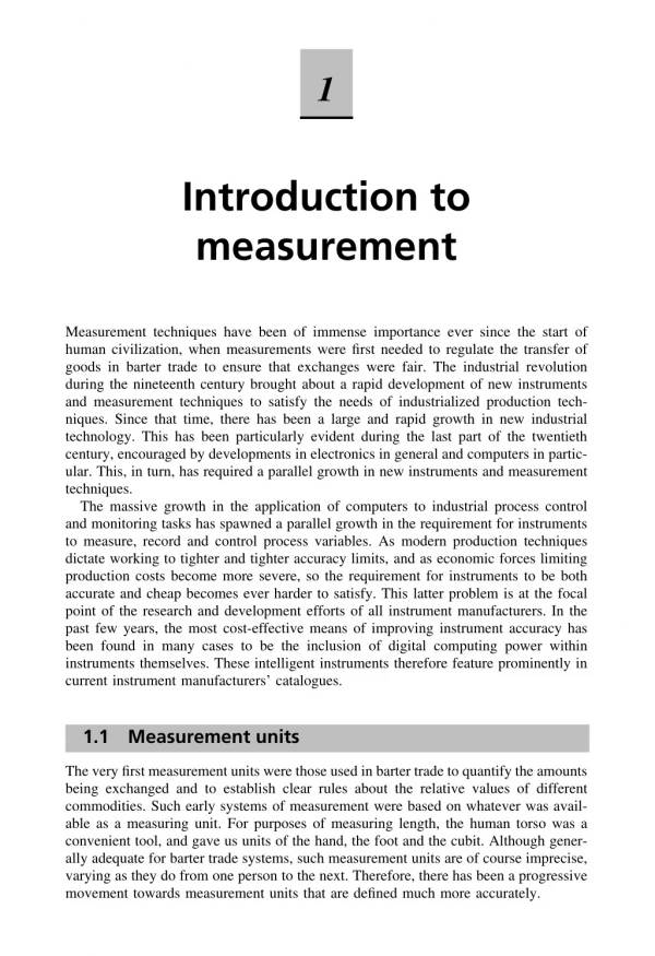
1. 1 Introduction to measurement Measurement techniques have been of immense importance ever since the start of human civilization, when measurements were first needed to regulate the transfer of goods in barter trade to ensure that exchanges were fair. The industrial revolution during the nineteenth century brought about a rapid development of new instruments and measurement techniques to satisfy the needs of industrialized production tech- niques. Since that time, there has been a large and rapid growth in new industrial technology. This has been particularly evident during the last part of the twentieth century, encouraged by developments in electronics in general and computers in partic- ular. This, in turn, has required a parallel growth in new instruments and measurement techniques. The massive growth in the application of computers to industrial process control and monitoring tasks has spawned a parallel growth in the requirement for instruments to measure, record and control process variables. As modern production techniques dictate working to tighter and tighter accuracy limits, and as economic forces limiting production costs become more severe, so the requirement for instruments to be both accurate and cheap becomes ever harder to satisfy. This latter problem is at the focal point of the research and development efforts of all instrument manufacturers. In the past few years, the most cost-effective means of improving instrument accuracy has been found in many cases to be the inclusion of digital computing power within instruments themselves. These intelligent instruments therefore feature prominently in current instrument manufacturers’ catalogues. 1.1 Measurement units The very first measurement units were those used in barter trade to quantify the amounts being exchanged and to establish clear rules about the relative values of different commodities. Such early systems of measurement were based on whatever was avail- able as a measuring unit. For purposes of measuring length, the human torso was a convenient tool, and gave us units of the hand, the foot and the cubit. Although gener- ally adequate for barter trade systems, such measurement units are of course imprecise, varying as they do from one person to the next. Therefore, there has been a progressive movement towards measurement units that are defined much more accurately.

2. Introduction to measurement 4 The first improved measurement unit was a unit of length (the metre) defined as 10?7times the polar quadrant of the earth. A platinum bar made to this length was established as a standard of length in the early part of the nineteenth century. This was superseded by a superior quality standard bar in 1889, manufactured from a platinum–iridium alloy. Since that time, technological research has enabled further improvements to be made in the standard used for defining length. Firstly, in 1960, a standard metre was redefined in terms of 1.65076373 ð 106wavelengths of the radia- tion from krypton-86 in vacuum. More recently, in 1983, the metre was redefined yet again as the length of path travelled by light in an interval of 1/299792458 seconds. In a similar fashion, standard units for the measurement of other physical quantities have been defined and progressively improved over the years. The latest standards for defining the units used for measuring a range of physical variables are given in Table 1.1. The early establishment of standards for the measurement of physical quantities proceeded in several countries at broadly parallel times, and in consequence, several sets of units emerged for measuring the same physical variable. For instance, length can be measured in yards, metres, or several other units. Apart from the major units of length, subdivisions of standard units exist such as feet, inches, centimetres and millimetres, with a fixed relationship between each fundamental unit and its sub- divisions. Table 1.1 Definitions of standard units Physical quantity Standard unit Definition Length metre The length of path travelled by light in an interval of 1/299 792 458 seconds The mass of a platinum–iridium cylinder kept in the International Bureau of Weights and Measures, S` evres, Paris 9.192631770 ð 109cycles of radiation from vaporized caesium-133 (an accuracy of 1 in 1012or 1 second in 36 000 years) The temperature difference between absolute zero and the triple point of water is defined as 273.16 kelvin One ampere is the current flowing through two infinitely long parallel conductors of negligible cross-section placed 1 metre apart in a vacuum and producing a force of 2 ð 10?7newtons per metre length of conductor One candela is the luminous intensity in a given direction from a source emitting monochromatic radiation at a frequency of 540 terahertz (Hz ð 1012) and with a radiant density in that direction of 1.4641 mW/steradian. (1 steradian is the solid angle which, having its vertex at the centre of a sphere, cuts off an area of the sphere surface equal to that of a square with sides of length equal to the sphere radius) The number of atoms in a 0.012kg mass of carbon-12 Mass kilogram Time second Temperature kelvin Current ampere Luminous intensity candela Matter mole

3. Measurement and Instrumentation Principles 5 Table 1.2 Fundamental and derived SI units (a) Fundamental units Quantity Standard unit Symbol Length Mass Time Electric current Temperature Luminous intensity Matter metre kilogram second ampere kelvin candela mole m kg s A K cd mol (b) Supplementary fundamental units Quantity Standard unit Symbol Plane angle Solid angle radian steradian rad sr (c) Derived units Derivation formula Quantity Standard unit Symbol m2 m3 m/s m/s2 rad/s rad/s2 kg/m3 m3/kg kg/s m3/s N N/m2 Nm kgm/s kgm2 m2/s Ns/m2 J J/m3 W W/mK C V V/m ? F H S ?m F/m H/m A/m2 Area Volume Velocity Acceleration Angular velocity Angular acceleration Density Specific volume Mass flow rate Volume flow rate Force Pressure Torque Momentum Moment of inertia Kinematic viscosity Dynamic viscosity Work, energy, heat Specific energy Power Thermal conductivity Electric charge Voltage, e.m.f., pot. diff. Electric field strength Electric resistance Electric capacitance Electric inductance Electric conductance Resistivity Permittivity Permeability Current density square metre cubic metre metre per second metre per second squared radian per second radian per second squared kilogram per cubic metre cubic metre per kilogram kilogram per second cubic metre per second newton newton per square metre newton metre kilogram metre per second kilogram metre squared square metre per second newton second per square metre joule joule per cubic metre watt watt per metre kelvin coulomb volt volt per metre ohm farad henry siemen ohm metre farad per metre henry per metre ampere per square metre kgm/s2 Nm J/s As W/A V/A As/V Vs/A A/V (continued overleaf )

4. Introduction to measurement 6 Table 1.2 (continued) (c) Derived units Derivation formula Quantity Standard unit Symbol Magnetic flux Magnetic flux density Magnetic field strength Frequency Luminous flux Luminance Illumination Molar volume Molarity Molar energy weber tesla ampere per metre hertz lumen candela per square metre lux cubic metre per mole mole per kilogram joule per mole Wb T A/m Hz lm cd/m2 lx m3/mol mol/kg J/mol Vs Wb/m2 s?1 cdsr lm/m2 Yards, feet and inches belong to the Imperial System of units, which is characterized by having varying and cumbersome multiplication factors relating fundamental units to subdivisions such as 1760 (miles to yards), 3 (yards to feet) and 12 (feet to inches). The metric system is an alternative set of units, which includes for instance the unit of the metre and its centimetre and millimetre subdivisions for measuring length. All multiples and subdivisions of basic metric units are related to the base by factors of ten and such units are therefore much easier to use than Imperial units. However, in the case of derived units such as velocity, the number of alternative ways in which these can be expressed in the metric system can lead to confusion. As a result of this, an internationally agreed set of standard units (SI units or Syst` emes Internationales d’Unit´ es) has been defined, and strong efforts are being made to encourage the adoption of this system throughout the world. In support of this effort, the SI system of units will be used exclusively in this book. However, it should be noted that the Imperial system is still widely used, particularly in America and Britain. The European Union has just deferred planned legislation to ban the use of Imperial units in Europe in the near future, and the latest proposal is to introduce such legislation to take effect from the year 2010. The full range of fundamental SI measuring units and the further set of units derived from them are given in Table 1.2. Conversion tables relating common Imperial and metric units to their equivalent SI units can also be found in Appendix 1. 1.2 Measurement system applications Today, the techniques of measurement are of immense importance in most facets of human civilization. Present-day applications of measuring instruments can be classi- fied into three major areas. The first of these is their use in regulating trade, applying instruments that measure physical quantities such as length, volume and mass in terms of standard units. The particular instruments and transducers employed in such appli- cations are included in the general description of instruments presented in Part 2 of this book.

5. Measurement and Instrumentation Principles 7 The second application area of measuring instruments is in monitoring functions. These provide information that enables human beings to take some prescribed action accordingly. The gardener uses a thermometer to determine whether he should turn the heat on in his greenhouse or open the windows if it is too hot. Regular study of a barometer allows us to decide whether we should take our umbrellas if we are planning to go out for a few hours. Whilst there are thus many uses of instrumentation in our normal domestic lives, the majority of monitoring functions exist to provide the information necessary to allow a human being to control some industrial operation or process. In a chemical process for instance, the progress of chemical reactions is indicated by the measurement of temperatures and pressures at various points, and such measurements allow the operator to take correct decisions regarding the electrical supply to heaters, cooling water flows, valve positions etc. One other important use of monitoring instruments is in calibrating the instruments used in the automatic process control systems described below. Use as part of automatic feedback control systems forms the third application area of measurement systems. Figure 1.1 shows a functional block diagram of a simple temperature control system in which the temperature Ta of a room is maintained at a reference value Td. The value of the controlled variable Ta, as determined by a temperature-measuring device, is compared with the reference value Td, and the differ- ence e is applied as an error signal to the heater. The heater then modifies the room temperature until TaD Td. The characteristics of the measuring instruments used in any feedback control system are of fundamental importance to the quality of control achieved. The accuracy and resolution with which an output variable of a process is controlled can never be better than the accuracy and resolution of the measuring instruments used. This is a very important principle, but one that is often inadequately discussed in many texts on automatic control systems. Such texts explore the theoret- ical aspects of control system design in considerable depth, but fail to give sufficient emphasis to the fact that all gain and phase margin performance calculations etc. are entirely dependent on the quality of the process measurements obtained. Comparator Heater Room Reference value Td Error signal Room temperature (Td−Ta) Ta Ta Temperature measuring device Fig. 1.1 Elements of a simple closed-loop control system.

6. Introduction to measurement 8 1.3 Elements of a measurement system A measuring system exists to provide information about the physical value of some variable being measured. In simple cases, the system can consist of only a single unit that gives an output reading or signal according to the magnitude of the unknown variable applied to it. However, in more complex measurement situations, a measuring system consists of several separate elements as shown in Figure 1.2. These compo- nents might be contained within one or more boxes, and the boxes holding individual measurement elements might be either close together or physically separate. The term measuring instrument is commonly used to describe a measurement system, whether it contains only one or many elements, and this term will be widely used throughout this text. The first element in any measuring system is the primary sensor: this gives an output that is a function of the measurand (the input applied to it). For most but not all sensors, this function is at least approximately linear. Some examples of primary sensors are a liquid-in-glass thermometer, a thermocouple and a strain gauge. In the case of the mercury-in-glass thermometer, the output reading is given in terms of the level of the mercury, and so this particular primary sensor is also a complete measurement system in itself. However, in general, the primary sensor is only part of a measurement system. The types of primary sensors available for measuring a wide range of physical quantities are presented in Part 2 of this book. Variable conversion elements are needed where the output variable of a primary transducer is in an inconvenient form and has to be converted to a more convenient form. For instance, the displacement-measuring strain gauge has an output in the form of a varying resistance. The resistance change cannot be easily measured and so it is converted to a change in voltage by a bridge circuit, which is a typical example of a variable conversion element. In some cases, the primary sensor and variable conversion element are combined, and the combination is known as a transducer.Ł Signal processing elements exist to improve the quality of the output of a measure- ment system in some way. A very common type of signal processing element is the electronic amplifier, which amplifies the output of the primary transducer or variable conversion element, thus improving the sensitivity and resolution of measurement. This element of a measuring system is particularly important where the primary transducer has a low output. For example, thermocouples have a typical output of only a few millivolts. Other types of signal processing element are those that filter out induced noise and remove mean levels etc. In some devices, signal processing is incorporated into a transducer, which is then known as a transmitter.Ł In addition to these three components just mentioned, some measurement systems have one or two other components, firstly to transmit the signal to some remote point and secondly to display or record the signal if it is not fed automatically into a feed- back control system. Signal transmission is needed when the observation or application point of the output of a measurement system is some distance away from the site of the primary transducer. Sometimes, this separation is made solely for purposes of convenience, but more often it follows from the physical inaccessibility or envi- ronmental unsuitability of the site of the primary transducer for mounting the signal ŁIn some cases, the word ‘sensor’ is used generically to refer to both transducers and transmitters.

7. Measurement and Instrumentation Principles 9 Measured variable (measurand) Output measurement Variable conversion element Sensor Signal processing Output display/ recording Use of measurement at remote point Signal transmission Signal presentation or recording Fig. 1.2 Elements of a measuring instrument. presentation/recording unit. The signal transmission element has traditionally consisted of single or multi-cored cable, which is often screened to minimize signal corruption by induced electrical noise. However, fibre-optic cables are being used in ever increasing numbers in modern installations, in part because of their low transmission loss and imperviousness to the effects of electrical and magnetic fields. The final optional element in a measurement system is the point where the measured signal is utilized. In some cases, this element is omitted altogether because the measure- ment is used as part of an automatic control scheme, and the transmitted signal is fed directly into the control system. In other cases, this element in the measurement system takes the form either of a signal presentation unit or of a signal-recording unit. These take many forms according to the requirements of the particular measurement application, and the range of possible units is discussed more fully in Chapter 11. 1.4 Choosing appropriate measuring instruments The starting point in choosing the most suitable instrument to use for measurement of a particular quantity in a manufacturing plant or other system is the specification of the instrument characteristics required, especially parameters like the desired measure- ment accuracy, resolution, sensitivity and dynamic performance (see next chapter for definitions of these). It is also essential to know the environmental conditions that the instrument will be subjected to, as some conditions will immediately either eliminate the possibility of using certain types of instrument or else will create a requirement for expensive protection of the instrument. It should also be noted that protection reduces the performance of some instruments, especially in terms of their dynamic charac- teristics (for example, sheaths protecting thermocouples and resistance thermometers reduce their speed of response). Provision of this type of information usually requires the expert knowledge of personnel who are intimately acquainted with the operation of the manufacturing plant or system in question. Then, a skilled instrument engineer, having knowledge of all the instruments that are available for measuring the quantity in question, will be able to evaluate the possible list of instruments in terms of their accuracy, cost and suitability for the environmental conditions and thus choose the

8. Introduction to measurement 10 most appropriate instrument. As far as possible, measurement systems and instruments should be chosen that are as insensitive as possible to the operating environment, although this requirement is often difficult to meet because of cost and other perfor- mance considerations. The extent to which the measured system will be disturbed during the measuring process is another important factor in instrument choice. For example, significant pressure loss can be caused to the measured system in some techniques of flow measurement. Published literature is of considerable help in the choice of a suitable instrument for a particular measurement situation. Many books are available that give valuable assistance in the necessary evaluation by providing lists and data about all the instru- ments available for measuring a range of physical quantities (e.g. Part 2 of this text). However, new techniques and instruments are being developed all the time, and there- fore a good instrumentation engineer must keep abreast of the latest developments by reading the appropriate technical journals regularly. The instrument characteristics discussed in the next chapter are the features that form the technical basis for a comparison between the relative merits of different instruments. Generally, the better the characteristics, the higher the cost. However, in comparing the cost and relative suitability of different instruments for a particular measurement situation, considerations of durability, maintainability and constancy of performance are also very important because the instrument chosen will often have to be capable of operating for long periods without performance degradation and a requirement for costly maintenance. In consequence of this, the initial cost of an instrument often has a low weighting in the evaluation exercise. Cost is very strongly correlated with the performance of an instrument, as measured by its static characteristics. Increasing the accuracy or resolution of an instrument, for example, can only be done at a penalty of increasing its manufacturing cost. Instru- ment choice therefore proceeds by specifying the minimum characteristics required by a measurement situation and then searching manufacturers’ catalogues to find an instrument whose characteristics match those required. To select an instrument with characteristics superior to those required would only mean paying more than necessary for a level of performance greater than that needed. As well as purchase cost, other important factors in the assessment exercise are instrument durability and the maintenance requirements. Assuming that one had £10000 to spend, one would not spend £8000 on a new motor car whose projected life was five years if a car of equivalent specification with a projected life of ten years was available for £10000. Likewise, durability is an important consideration in the choice of instruments. The projected life of instruments often depends on the conditions in which the instrument will have to operate. Maintenance requirements must also be taken into account, as they also have cost implications. As a general rule, a good assessment criterion is obtained if the total purchase cost and estimated maintenance costs of an instrument over its life are divided by the period of its expected life. The figure obtained is thus a cost per year. However, this rule becomes modified where instruments are being installed on a process whose life is expected to be limited, perhaps in the manufacture of a particular model of car. Then, the total costs can only be divided by the period of time that an instrument is expected to be used for, unless an alternative use for the instrument is envisaged at the end of this period.

9. Measurement and Instrumentation Principles 11 To summarize therefore, instrument choice is a compromise between performance characteristics, ruggedness and durability, maintenance requirements and purchase cost. To carry out such an evaluation properly, the instrument engineer must have a wide knowledge of the range of instruments available for measuring particular physical quan- tities, and he/she must also have a deep understanding of how instrument characteristics are affected by particular measurement situations and operating conditions.

10. 2 Instrument types and performance characteristics 2.1 Review of instrument types Instruments can be subdivided into separate classes according to several criteria. These subclassifications are useful in broadly establishing several attributes of particular instruments such as accuracy, cost, and general applicability to different applications. 2.1.1 Active and passive instruments Instruments are divided into active or passive ones according to whether the instrument output is entirely produced by the quantity being measured or whether the quantity being measured simply modulates the magnitude of some external power source. This is illustrated by examples. An example of a passive instrument is the pressure-measuring device shown in Figure 2.1. The pressure of the fluid is translated into a movement of a pointer against a scale. The energy expended in moving the pointer is derived entirely from the change in pressure measured: there are no other energy inputs to the system. An example of an active instrument is a float-type petrol tank level indicator as sketched in Figure 2.2. Here, the change in petrol level moves a potentiometer arm, and the output signal consists of a proportion of the external voltage source applied across the two ends of the potentiometer. The energy in the output signal comes from the external power source: the primary transducer float system is merely modulating the value of the voltage from this external power source. In active instruments, the external power source is usually in electrical form, but in some cases, it can be other forms of energy such as a pneumatic or hydraulic one. One very important difference between active and passive instruments is the level of measurement resolution that can be obtained. With the simple pressure gauge shown, the amount of movement made by the pointer for a particular pressure change is closely defined by the nature of the instrument. Whilst it is possible to increase measurement resolution by making the pointer longer, such that the pointer tip moves through a longer arc, the scope for such improvement is clearly restricted by the practical limit of how long the pointer can conveniently be. In an active instrument, however, adjust- ment of the magnitude of the external energy input allows much greater control over

11. Measurement and Instrumentation Principles 13 Pointer Scale Spring Piston Pivot Fluid Fig. 2.1 Passive pressure gauge. Pivot Float Output voltage Fig. 2.2 Petrol-tank level indicator. measurement resolution. Whilst the scope for improving measurement resolution is much greater incidentally, it is not infinite because of limitations placed on the magni- tude of the external energy input, in consideration of heating effects and for safety reasons. In terms of cost, passive instruments are normally of a more simple construction than active ones and are therefore cheaper to manufacture. Therefore, choice between active and passive instruments for a particular application involves carefully balancing the measurement resolution requirements against cost. 2.1.2 Null-type and deflection-type instruments The pressure gauge just mentioned is a good example of a deflection type of instrument, where the value of the quantity being measured is displayed in terms of the amount of

12. Instrument types and performance characteristics 14 Weights Piston Datum level Fig. 2.3 Deadweight pressure gauge. movement of a pointer. An alternative type of pressure gauge is the deadweight gauge shown in Figure 2.3, which is a null-type instrument. Here, weights are put on top of the piston until the downward force balances the fluid pressure. Weights are added until the piston reaches a datum level, known as the null point. Pressure measurement is made in terms of the value of the weights needed to reach this null position. The accuracy of these two instruments depends on different things. For the first one it depends on the linearity and calibration of the spring, whilst for the second it relies on the calibration of the weights. As calibration of weights is much easier than careful choice and calibration of a linear-characteristic spring, this means that the second type of instrument will normally be the more accurate. This is in accordance with the general rule that null-type instruments are more accurate than deflection types. In terms of usage, the deflection type instrument is clearly more convenient. It is far simpler to read the position of a pointer against a scale than to add and subtract weights until a null point is reached. A deflection-type instrument is therefore the one that would normally be used in the workplace. However, for calibration duties, the null-type instrument is preferable because of its superior accuracy. The extra effort required to use such an instrument is perfectly acceptable in this case because of the infrequent nature of calibration operations. 2.1.3 Analogue and digital instruments An analogue instrument gives an output that varies continuously as the quantity being measured changes. The output can have an infinite number of values within the range that the instrument is designed to measure. The deflection-type of pressure gauge described earlier in this chapter (Figure 2.1) is a good example of an analogue instru- ment. As the input value changes, the pointer moves with a smooth continuous motion. Whilst the pointer can therefore be in an infinite number of positions within its range of movement, the number of different positions that the eye can discriminate between is strictly limited, this discrimination being dependent upon how large the scale is and how finely it is divided. A digital instrument has an output that varies in discrete steps and so can only have a finite number of values. The rev counter sketched in Figure 2.4 is an example of

13. Measurement and Instrumentation Principles 15 Switch Counter Cam Fig. 2.4 Rev counter. a digital instrument. A cam is attached to the revolving body whose motion is being measured, and on each revolution the cam opens and closes a switch. The switching operations are counted by an electronic counter. This system can only count whole revolutions and cannot discriminate any motion that is less than a full revolution. The distinction between analogue and digital instruments has become particularly important with the rapid growth in the application of microcomputers to automatic control systems. Any digital computer system, of which the microcomputer is but one example, performs its computations in digital form. An instrument whose output is in digital form is therefore particularly advantageous in such applications, as it can be interfaced directly to the control computer. Analogue instruments must be interfaced to the microcomputer by an analogue-to-digital (A/D) converter, which converts the analogue output signal from the instrument into an equivalent digital quantity that can be read into the computer. This conversion has several disadvantages. Firstly, the A/D converter adds a significant cost to the system. Secondly, a finite time is involved in the process of converting an analogue signal to a digital quantity, and this time can be critical in the control of fast processes where the accuracy of control depends on the speed of the controlling computer. Degrading the speed of operation of the control computer by imposing a requirement for A/D conversion thus impairs the accuracy by which the process is controlled. 2.1.4 Indicating instruments and instruments with a signal output The final way in which instruments can be divided is between those that merely give an audio or visual indication of the magnitude of the physical quantity measured and those that give an output in the form of a measurement signal whose magnitude is proportional to the measured quantity. The class of indicating instruments normally includes all null-type instruments and most passive ones. Indicators can also be further divided into those that have an analogue output and those that have a digital display. A common analogue indicator is the liquid-in-glass thermometer. Another common indicating device, which exists in both analogue and digital forms, is the bathroom scale. The older mechanical form of this is an analogue type of instrument that gives an output consisting of a rotating

14. Instrument types and performance characteristics 16 pointer moving against a scale (or sometimes a rotating scale moving against a pointer). More recent electronic forms of bathroom scale have a digital output consisting of numbers presented on an electronic display. One major drawback with indicating devices is that human intervention is required to read and record a measurement. This process is particularly prone to error in the case of analogue output displays, although digital displays are not very prone to error unless the human reader is careless. Instruments that have a signal-type output are commonly used as part of automatic control systems. In other circumstances, they can also be found in measurement systems where the output measurement signal is recorded in some way for later use. This subject is covered in later chapters. Usually, the measurement signal involved is an electrical voltage, but it can take other forms in some systems such as an electrical current, an optical signal or a pneumatic signal. 2.1.5 Smart and non-smart instruments The advent of the microprocessor has created a new division in instruments between those that do incorporate a microprocessor (smart) and those that don’t. Smart devices are considered in detail in Chapter 9. 2.2 Static characteristics of instruments If we have a thermometer in a room and its reading shows a temperature of 20°C, then it does not really matter whether the true temperature of the room is 19.5°C or 20.5°C. Such small variations around 20°C are too small to affect whether we feel warm enough or not. Our bodies cannot discriminate between such close levels of temperature and therefore a thermometer with an inaccuracy of š0.5°C is perfectly adequate. If we had to measure the temperature of certain chemical processes, however, a variation of 0.5°C might have a significant effect on the rate of reaction or even the products of a process. A measurement inaccuracy much less than š0.5°C is therefore clearly required. Accuracy of measurement is thus one consideration in the choice of instrument for a particular application. Other parameters such as sensitivity, linearity and the reaction to ambient temperature changes are further considerations. These attributes are collectively known as the static characteristics of instruments, and are given in the data sheet for a particular instrument. It is important to note that the values quoted for instrument characteristics in such a data sheet only apply when the instrument is used under specified standard calibration conditions. Due allowance must be made for variations in the characteristics when the instrument is used in other conditions. The various static characteristics are defined in the following paragraphs. 2.2.1 Accuracy and inaccuracy (measurement uncertainty) The accuracy of an instrument is a measure of how close the output reading of the instrument is to the correct value. In practice, it is more usual to quote the inaccuracy figure rather than the accuracy figure for an instrument. Inaccuracy is the extent to

15. Measurement and Instrumentation Principles 17 which a reading might be wrong, and is often quoted as a percentage of the full-scale (f.s.) reading of an instrument. If, for example, a pressure gauge of range 0–10 bar has a quoted inaccuracy of š1.0% f.s. (š1% of full-scale reading), then the maximum error to be expected in any reading is 0.1 bar. This means that when the instrument is reading 1.0 bar, the possible error is 10% of this value. For this reason, it is an important system design rule that instruments are chosen such that their range is appropriate to the spread of values being measured, in order that the best possible accuracy is maintained in instrument readings. Thus, if we were measuring pressures with expected values between 0 and 1 bar, we would not use an instrument with a range of 0–10 bar. The term measurement uncertainty is frequently used in place of inaccuracy. 2.2.2 Precision/repeatability/reproducibility Precision is a term that describes an instrument’s degree of freedom from random errors. If a large number of readings are taken of the same quantity by a high precision instrument, then the spread of readings will be very small. Precision is often, though incorrectly, confused with accuracy. High precision does not imply anything about measurement accuracy. A high precision instrument may have a low accuracy. Low accuracy measurements from a high precision instrument are normally caused by a bias in the measurements, which is removable by recalibration. The terms repeatability and reproducibility mean approximately the same but are applied in different contexts as given below. Repeatability describes the closeness of output readings when the same input is applied repetitively over a short period of time, with the same measurement conditions, same instrument and observer, same location and same conditions of use maintained throughout. Reproducibility describes the closeness of output readings for the same input when there are changes in the method of measurement, observer, measuring instrument, location, conditions of use and time of measurement. Both terms thus describe the spread of output readings for the same input. This spread is referred to as repeatability if the measurement conditions are constant and as reproducibility if the measurement conditions vary. The degree of repeatability or reproducibility in measurements from an instrument is an alternative way of expressing its precision. Figure 2.5 illustrates this more clearly. The figure shows the results of tests on three industrial robots that were programmed to place components at a particular point on a table. The target point was at the centre of the concentric circles shown, and the black dots represent the points where each robot actually deposited components at each attempt. Both the accuracy and precision of Robot 1 are shown to be low in this trial. Robot 2 consistently puts the component down at approximately the same place but this is the wrong point. Therefore, it has high precision but low accuracy. Finally, Robot 3 has both high precision and high accuracy, because it consistently places the component at the correct target position. 2.2.3 Tolerance Tolerance is a term that is closely related to accuracy and defines the maximum error that is to be expected in some value. Whilst it is not, strictly speaking, a static

16. Instrument types and performance characteristics 18 (a) Low precision, low accuracy ROBOT 1 (b) High precision, low accuracy ROBOT 2 (c) High precision, high accuracy ROBOT 3 Fig. 2.5 Comparison of accuracy and precision. characteristic of measuring instruments, it is mentioned here because the accuracy of some instruments is sometimes quoted as a tolerance figure. When used correctly, tolerance describes the maximum deviation of a manufactured component from some specified value. For instance, crankshafts are machined with a diameter tolerance quoted as so many microns (10?6m), and electric circuit components such as resistors have tolerances of perhaps 5%. One resistor chosen at random from a batch having a nominal value 1000W and tolerance 5% might have an actual value anywhere between 950W and 1050W. 2.2.4 Range or span The range or span of an instrument defines the minimum and maximum values of a quantity that the instrument is designed to measure.

17. Measurement and Instrumentation Principles 19 2.2.5 Linearity It is normally desirable that the output reading of an instrument is linearly proportional to the quantity being measured. The Xs marked on Figure 2.6 show a plot of the typical output readings of an instrument when a sequence of input quantities are applied to it. Normal procedure is to draw a good fit straight line through the Xs, as shown in Figure 2.6. (Whilst this can often be done with reasonable accuracy by eye, it is always preferable to apply a mathematical least-squares line-fitting technique, as described in Chapter 11.) The non-linearity is then defined as the maximum deviation of any of the output readings marked X from this straight line. Non-linearity is usually expressed as a percentage of full-scale reading. 2.2.6 Sensitivity of measurement The sensitivity of measurement is a measure of the change in instrument output that occurs when the quantity being measured changes by a given amount. Thus, sensitivity is the ratio: scale deflection value of measurand producing deflection The sensitivity of measurement is therefore the slope of the straight line drawn on Figure 2.6. If, for example, a pressure of 2 bar produces a deflection of 10 degrees in a pressure transducer, the sensitivity of the instrument is 5 degrees/bar (assuming that the deflection is zero with zero pressure applied). Output reading Gradient = Sensitivity of measurement Measured quantity Fig. 2.6 Instrument output characteristic.

18. Instrument types and performance characteristics 20 Example 2.1 The following resistance values of a platinum resistance thermometer were measured at a range of temperatures. Determine the measurement sensitivity of the instrument in ohms/°C. Temperature (°C) Resistance (?) 307 314 321 328 200 230 260 290 Solution If these values are plotted on a graph, the straight-line relationship between resistance change and temperature change is obvious. For a change in temperature of 30°C, the change in resistance is 7?. Hence the measurement sensitivity D 7/30 D 0.233?/°C. 2.2.7 Threshold If the input to an instrument is gradually increased from zero, the input will have to reach a certain minimum level before the change in the instrument output reading is of a large enough magnitude to be detectable. This minimum level of input is known as the threshold of the instrument. Manufacturers vary in the way that they specify threshold for instruments. Some quote absolute values, whereas others quote threshold as a percentage of full-scale readings. As an illustration, a car speedometer typically has a threshold of about 15 km/h. This means that, if the vehicle starts from rest and acceler- ates, no output reading is observed on the speedometer until the speed reaches 15 km/h. 2.2.8 Resolution When an instrument is showing a particular output reading, there is a lower limit on the magnitude of the change in the input measured quantity that produces an observable change in the instrument output. Like threshold, resolution is sometimes specified as an absolute value and sometimes as a percentage of f.s. deflection. One of the major factors influencing the resolution of an instrument is how finely its output scale is divided into subdivisions. Using a car speedometer as an example again, this has subdivisions of typically 20 km/h. This means that when the needle is between the scale markings, we cannot estimate speed more accurately than to the nearest 5 km/h. This figure of 5 km/h thus represents the resolution of the instrument. 2.2.9 Sensitivity to disturbance All calibrations and specifications of an instrument are only valid under controlled conditions of temperature, pressure etc. These standard ambient conditions are usually defined in the instrument specification. As variations occur in the ambient temperature

19. Measurement and Instrumentation Principles 21 etc., certain static instrument characteristics change, and the sensitivity to disturbance is a measure of the magnitude of this change. Such environmental changes affect instruments in two main ways, known as zero drift and sensitivity drift. Zero drift is sometimes known by the alternative term, bias. Zero drift or bias describes the effect where the zero reading of an instrument is modified by a change in ambient conditions. This causes a constant error that exists over the full range of measurement of the instrument. The mechanical form of bathroom scale is a common example of an instrument that is prone to bias. It is quite usual to find that there is a reading of perhaps 1 kg with no one stood on the scale. If someone of known weight 70 kg were to get on the scale, the reading would be 71 kg, and if someone of known weight 100 kg were to get on the scale, the reading would be 101 kg. Zero drift is normally removable by calibration. In the case of the bathroom scale just described, a thumbwheel is usually provided that can be turned until the reading is zero with the scales unloaded, thus removing the bias. Zero drift is also commonly found in instruments like voltmeters that are affected by ambient temperature changes. Typical units by which such zero drift is measured are volts/°C. This is often called the zero drift coefficient related to temperature changes. If the characteristic of an instrument is sensitive to several environmental parameters, then it will have several zero drift coefficients, one for each environmental parameter. A typical change in the output characteristic of a pressure gauge subject to zero drift is shown in Figure 2.7(a). Sensitivity drift (also known as scale factor drift) defines the amount by which an instrument’s sensitivity of measurement varies as ambient conditions change. It is quantified by sensitivity drift coefficients that define how much drift there is for a unit change in each environmental parameter that the instrument characteristics are sensitive to. Many components within an instrument are affected by environmental fluctuations, such as temperature changes: for instance, the modulus of elasticity of a spring is temperature dependent. Figure 2.7(b) shows what effect sensitivity drift can have on the output characteristic of an instrument. Sensitivity drift is measured in units of the form (angular degree/bar)/°C. If an instrument suffers both zero drift and sensitivity drift at the same time, then the typical modification of the output characteristic is shown in Figure 2.7(c). Example 2.2 A spring balance is calibrated in an environment at a temperature of 20°C and has the following deflection/load characteristic. Load (kg) Deflection (mm) 0 0 1 2 3 20 40 60 It is then used in an environment at a temperature of 30°C and the following deflec- tion/load characteristic is measured. Load (kg): Deflection (mm) 0 5 1 2 3 27 49 71 Determine the zero drift and sensitivity drift per°C change in ambient temperature.

20. Instrument types and performance characteristics 22 Scale reading Scale reading Characteristic with zero drift Characteristic with sensitivity drift Nominal characteristic Nominal characteristic Pressure Pressure (a) (b) Scale reading Characteristic with zero drift and sensitivity drift Nominal characteristic Pressure (c) Fig. 2.7 Effects of disturbance: (a) zero drift; (b) sensitivity drift; (c) zero drift plus sensitivity drift. Solution At 20°C, deflection/load characteristic is a straight line. Sensitivity D 20mm/kg. At 30°C, deflection/load characteristic is still a straight line. Sensitivity D 22mm/kg. Bias (zero drift) D 5mm (the no-load deflection) Sensitivity drift D 2mm/kg Zero drift/°C D 5/10 D 0.5mm/°C Sensitivity drift/°C D 2/10 D 0.2 (mm per kg)/°C 2.2.10 Hysteresis effects Figure 2.8 illustrates the output characteristic of an instrument that exhibits hysteresis. If the input measured quantity to the instrument is steadily increased from a negative value, the output reading varies in the manner shown in curve (a). If the input variable is then steadily decreased, the output varies in the manner shown in curve (b). The non-coincidence between these loading and unloading curves is known as hysteresis. Two quantities are defined, maximum input hysteresis and maximum output hysteresis, as shown in Figure 2.8. These are normally expressed as a percentage of the full-scale input or output reading respectively.

21. Measurement and Instrumentation Principles Curve B − variable decreasing 23 Output reading Maximum output hysteresis Curve A − variable increasing Measured variable Maximum input hysteresis Dead space Fig. 2.8 Instrument characteristic with hysteresis. Hysteresis is most commonly found in instruments that contain springs, such as the passive pressure gauge (Figure 2.1) and the Prony brake (used for measuring torque). It is also evident when friction forces in a system have different magnitudes depending on the direction of movement, such as in the pendulum-scale mass-measuring device. Devices like the mechanical flyball (a device for measuring rotational velocity) suffer hysteresis from both of the above sources because they have friction in moving parts and also contain a spring. Hysteresis can also occur in instruments that contain electrical windings formed round an iron core, due to magnetic hysteresis in the iron. This occurs in devices like the variable inductance displacement transducer, the LVDT and the rotary differential transformer. 2.2.11 Dead space Dead space is defined as the range of different input values over which there is no change in output value. Any instrument that exhibits hysteresis also displays dead space, as marked on Figure 2.8. Some instruments that do not suffer from any signif- icant hysteresis can still exhibit a dead space in their output characteristics, however. Backlash in gears is a typical cause of dead space, and results in the sort of instrument output characteristic shown in Figure 2.9. Backlash is commonly experienced in gear- sets used to convert between translational and rotational motion (which is a common technique used to measure translational velocity). 2.3 Dynamic characteristics of instruments The static characteristics of measuring instruments are concerned only with the steady- state reading that the instrument settles down to, such as the accuracy of the reading etc.

22. Instrument types and performance characteristics 24 Output reading + − + Measured variable Dead space − Fig. 2.9 Instrument characteristic with dead space. The dynamic characteristics of a measuring instrument describe its behaviour between the time a measured quantity changes value and the time when the instrument output attains a steady value in response. As with static characteristics, any values for dynamic characteristics quoted in instrument data sheets only apply when the instrument is used under specified environmental conditions. Outside these calibration conditions, some variation in the dynamic parameters can be expected. In any linear, time-invariant measuring system, the following general relation can be written between input and output for time ?t? > 0: dtnC an?1dn?1q0 D bmdmqi andnq0 dtn?1C ÐÐÐ C a1dq0 dtmC bm?1dm?1qi C a0q0 dt dtm?1C ÐÐÐ C b1dqi ?2.1? C b0qi dt where qiis the measured quantity, q0is the output reading and a0...an, b0...bmare constants. The reader whose mathematical background is such that the above equation appears daunting should not worry unduly, as only certain special, simplified cases of it are applicable in normal measurement situations. The major point of importance is to have a practical appreciation of the manner in which various different types of instrument respond when the measurand applied to them varies. If we limit consideration to that of step changes in the measured quantity only, then equation (2.1) reduces to: dtnC an?1dn?1q0 andnq0 dtn?1C ÐÐÐ C a1dq0 ?2.2? C a0q0D b0qi dt

23. Measurement and Instrumentation Principles 25 Further simplification can be made by taking certain special cases of equation (2.2), which collectively apply to nearly all measurement systems. 2.3.1 Zero order instrument If all the coefficients a1...another than a0in equation (2.2) are assumed zero, then: or ?2.3? a0q0D b0qi q0D b0qi/a0D Kqi where K is a constant known as the instrument sensitivity as defined earlier. Any instrument that behaves according to equation (2.3) is said to be of zero order type. Following a step change in the measured quantity at time t, the instrument output moves immediately to a new value at the same time instant t, as shown in Figure 2.10. A potentiometer, which measures motion, is a good example of such an instrument, where the output voltage changes instantaneously as the slider is displaced along the potentiometer track. 2.3.2 First order instrument If all the coefficients a2...an except for a0 and a1 are assumed zero in equation (2.2) then: a1dq0 dt Any instrument that behaves according to equation (2.4) is known as a first order instrument. If d/dt is replaced by the D operator in equation (2.4), we get: ?2.4? C a0q0D b0qi ?b0/a0?qi [1 C ?a1/a0?D] and rearranging this then gives ?2.5? a1Dq0C a0q0D b0qi q0D Measured quantity 0 t Time Instrument output 0 t Time Fig. 2.10 Zero order instrument characteristic.

24. Instrument types and performance characteristics 26 Defining K D b0/a0as the static sensitivity and ? D a1/a0as the time constant of the system, equation (2.5) becomes: Kqi 1 C ?D ?2.6? q0D If equation (2.6) is solved analytically, the output quantity q0 in response to a step change in qiat time t varies with time in the manner shown in Figure 2.11. The time constant ? of the step response is the time taken for the output quantity q0to reach 63% of its final value. The liquid-in-glass thermometer (see Chapter 14) is a good example of a first order instrument. It is well known that, if a thermometer at room temperature is plunged into boiling water, the output e.m.f. does not rise instantaneously to a level indicating 100°C, but instead approaches a reading indicating 100°C in a manner similar to that shown in Figure 2.11. A large number of other instruments also belong to this first order class: this is of particular importance in control systems where it is necessary to take account of the time lag that occurs between a measured quantity changing in value and the measuring instrument indicating the change. Fortunately, the time constant of many first order instruments is small relative to the dynamics of the process being measured, and so no serious problems are created. Example 2.3 A balloon is equipped with temperature and altitude measuring instruments and has radio equipment that can transmit the output readings of these instruments back to ground. The balloon is initially anchored to the ground with the instrument output readings in steady state. The altitude-measuring instrument is approximately zero order and the temperature transducer first order with a time constant of 15 seconds. The Magnitude Measured quantity Instrument output 63% τ 0 t (time constant) Time Fig. 2.11 First order instrument characteristic.

25. Measurement and Instrumentation Principles 27 temperature on the ground, T0, is 10°C and the temperature Tx at an altitude of x metres is given by the relation: TxD T0? 0.01x (a) If the balloon is released at time zero, and thereafter rises upwards at a velocity of 5 metres/second, draw a table showing the temperature and altitude measurements reported at intervals of 10 seconds over the first 50 seconds of travel. Show also in the table the error in each temperature reading. (b) What temperature does the balloon report at an altitude of 5000 metres? Solution In order to answer this question, it is assumed that the solution of a first order differ- ential equation has been presented to the reader in a mathematics course. If the reader is not so equipped, the following solution will be difficult to follow. Let the temperature reported by the balloon at some general time t be Tr. Then Tx is related to Trby the relation: 1 C ?DDT0? 0.01x D10 ? 0.01x 1 C 15D Tx TrD 1 C ?D It is given that x D 5t, thus: TrD10 ? 0.05t The transient or complementary function part of the solution (TxD 0) is given by: TrcfD Ce?t/15 The particular integral part of the solution is given by: TrpiD 10 ? 0.05?t ? 15? Thus, the whole solution is given by: TrD TrcfC TrpiD Ce?t/15C 10 ? 0.05?t ? 15? Applying initial conditions: At t D 0, TrD 10, i.e. 10 D Ce?0C 10 ? 0.05??15? Thus C D ?0.75 and therefore: TrD 10 ? 0.75e?t/15? 0.05?t ? 15? Using the above expression to calculate Trfor various values of t, the following table can be constructed: 1 C 15D Time Altitude Temperature reading Temperature error 0 0 10 0 0.36 0.55 0.65 0.70 0.72 10 20 30 40 50 50 100 150 200 250 9.86 9.55 9.15 8.70 8.22 (b) At 5000 m, t D 1000 seconds. Calculating Trfrom the above expression: TrD 10 ? 0.75e?1000/15? 0.05?1000 ? 15? The exponential term approximates to zero and so Trcan be written as: Tr³ 10 ? 0.05?985? D ?39.25°C This result might have been inferred from the table above where it can be seen that the error is converging towards a value of 0.75. For large values of t, the transducer reading lags the true temperature value by a period of time equal to the time constant of

26. Instrument types and performance characteristics 28 15 seconds. In this time, the balloon travels a distance of 75 metres and the temperature falls by 0.75°. Thus for large values of t, the output reading is always 0.75°less than it should be. 2.3.3 Second order instrument If all coefficients a3...another than a0, a1and a2in equation (2.2) are assumed zero, then we get: a2d2q0 dt Applying the D operator again: a2D2q0C a1Dq0C a0q0D b0qi, and rearranging: dt2C a1dq0 ?2.7? C a0q0D b0qi b0qi ?2.8? q0D a0C a1D C a2D2 It is convenient to re-express the variables a0, a1, a2and b0in equation (2.8) in terms of three parameters K (static sensitivity), ω (undamped natural frequency) and ? (damping ratio), where: K D b0/a0; Re-expressing equation (2.8) in terms of K, ω and ? we get: ω D a0/a2; ? D a1/2a0a2 q0 qi K ?2.9? D D2/ω2C 2?D/ω C 1 This is the standard equation for a second order system and any instrument whose response can be described by it is known as a second order instrument. If equation (2.9) is solved analytically, the shape of the step response obtained depends on the value of the damping ratio parameter ?. The output responses of a second order instrument for various values of ? following a step change in the value of the measured quantity at time t are shown in Figure 2.12. For case (A) where ? D 0, there is no damping and the instrument output exhibits constant amplitude oscillations when disturbed by any change in the physical quantity measured. For light damping of ? D 0.2, repre- sented by case (B), the response to a step change in input is still oscillatory but the oscillations gradually die down. Further increase in the value of ? reduces oscillations and overshoot still more, as shown by curves (C) and (D), and finally the response becomes very overdamped as shown by curve (E) where the output reading creeps up slowly towards the correct reading. Clearly, the extreme response curves (A) and (E) are grossly unsuitable for any measuring instrument. If an instrument were to be only ever subjected to step inputs, then the design strategy would be to aim towards a damping ratio of 0.707, which gives the critically damped response (C). Unfortunately, most of the physical quantities that instruments are required to measure do not change in the mathematically convenient form of steps, but rather in the form of ramps of varying slopes. As the form of the input variable changes, so the best value for ? varies, and choice of ? becomes one of compromise between those values that are best for each type of input variable behaviour anticipated. Commercial second order instruments, of which the accelerometer is a common example, are generally designed to have a damping ratio (?) somewhere in the range of 0.6–0.8.

27. Measurement and Instrumentation Principles 29 Magnitude A Measured quantity B C D E 0 t Time ε = 0.0 ε = 1.0 Output A Output D ε = 0.2 ε = 1.5 Output B Output E ε = 0.707 Output C Fig. 2.12 Response characteristics of second order instruments. 2.4 Necessity for calibration The foregoing discussion has described the static and dynamic characteristics of measur- ing instruments in some detail. However, an important qualification that has been omitted from this discussion is that an instrument only conforms to stated static and dynamic patterns of behaviour after it has been calibrated. It can normally be assumed that a new instrument will have been calibrated when it is obtained from an instrument manufacturer, and will therefore initially behave according to the characteristics stated in the specifications. During use, however, its behaviour will gradually diverge from the stated specification for a variety of reasons. Such reasons include mechanical wear, and the effects of dirt, dust, fumes and chemicals in the operating environment. The rate of divergence from standard specifications varies according to the type of instru- ment, the frequency of usage and the severity of the operating conditions. However, there will come a time, determined by practical knowledge, when the characteristics of the instrument will have drifted from the standard specification by an unacceptable amount. When this situation is reached, it is necessary to recalibrate the instrument to the standard specifications. Such recalibration is performed by adjusting the instrument

28. Instrument types and performance characteristics 30 at each point in its output range until its output readings are the same as those of a second standard instrument to which the same inputs are applied. This second instru- ment is one kept solely for calibration purposes whose specifications are accurately known. Calibration procedures are discussed more fully in Chapter 4. 2.5 Self-test questions 2.1 Explain what is meant by: (a) active instruments (b) passive instruments. Give examples of each and discuss the relative merits of these two classes of instruments. 2.2 Discuss the advantages and disadvantages of null and deflection types of measuring instrument. What are null types of instrument mainly used for and why? 2.3 Briefly define and explain all the static characteristics of measuring instruments. 2.4 Explain the difference between accuracy and precision in an instrument. 2.5 A tungsten/5% rhenium–tungsten/26% rhenium thermocouple has an output e.m.f. as shown in the following table when its hot (measuring) junction is at the temperatures shown. Determine the sensitivity of measurement for the thermocouple in mV/°C. mV °C 4.37 250 8.74 500 13.11 750 17.48 1000 2.6 Define sensitivity drift and zero drift. What factors can cause sensitivity drift and zero drift in instrument characteristics? 2.7 (a) An instrument is calibrated in an environment at a temperature of 20°C and the following output readings y are obtained for various input values x: 13.1 5 26.2 10 39.3 15 52.4 20 65.5 25 78.6 30 y x Determine the measurement sensitivity, expressed as the ratio y/x. (b) When the instrument is subsequently used in an environment at a temperature of 50°C, the input/output characteristic changes to the following: 14.7 5 29.4 10 44.1 15 58.8 20 73.5 25 88.2 30 y x Determine the new measurement sensitivity. Hence determine the sensitivity drift due to the change in ambient temperature of 30°C.

29. Measurement and Instrumentation Principles 31 2.8 A load cell is calibrated in an environment at a temperature of 21°C and has the following deflection/load characteristic: Load (kg) Deflection (mm) 0 50 1.0 100 2.0 150 3.0 200 4.0 0.0 When used in an environment at 35°C, its characteristic changes to the following: Load (kg) Deflection (mm) 0 50 1.3 100 2.4 150 3.5 200 4.6 0.2 (a) Determine the sensitivity at 21°C and 35°C. (b) Calculate the total zero drift and sensitivity drift at 35°C. (c) Hence determine the zero drift and sensitivity drift coefficients (in units of µm/°C and (µm per kg)/(°C)). 2.9 An unmanned submarine is equipped with temperature and depth measuring instruments and has radio equipment that can transmit the output readings of these instruments back to the surface. The submarine is initially floating on the surface of the sea with the instrument output readings in steady state. The depth- measuring instrument is approximately zero order and the temperature transducer first order with a time constant of 50 seconds. The water temperature on the sea surface, T0, is 20°C and the temperature Txat a depth of x metres is given by the relation: TxD T0? 0.01x (a) If the submarine starts diving at time zero, and thereafter goes down at a velocity of 0.5 metres/second, draw a table showing the temperature and depth measurements reported at intervals of 100 seconds over the first 500 seconds of travel. Show also in the table the error in each temperature reading. (b) What temperature does the submarine report at a depth of 1000 metres? 2.10 Write down the general differential equation describing the dynamic response of a second order measuring instrument and state the expressions relating the static sensitivity, undamped natural frequency and damping ratio to the parameters in this differential equation. Sketch the instrument response for the cases of heavy damping, critical damping and light damping, and state which of these is the usual target when a second order instrument is being designed.

30. 3 Errors during the measurement process 3.1 Introduction Errors in measurement systems can be divided into those that arise during the measure- ment process and those that arise due to later corruption of the measurement signal by induced noise during transfer of the signal from the point of measurement to some other point. This chapter considers only the first of these, with discussion on induced noise being deferred to Chapter 5. It is extremely important in any measurement system to reduce errors to the minimum possible level and then to quantify the maximum remaining error that may exist in any instrument output reading. However, in many cases, there is a further complication that the final output from a measurement system is calculated by combining together two or more measurements of separate physical variables. In this case, special consid- eration must also be given to determining how the calculated error levels in each separate measurement should be combined together to give the best estimate of the most likely error magnitude in the calculated output quantity. This subject is considered in section 3.6. The starting point in the quest to reduce the incidence of errors arising during the measurement process is to carry out a detailed analysis of all error sources in the system. Each of these error sources can then be considered in turn, looking for ways of eliminating or at least reducing the magnitude of errors. Errors arising during the measurement process can be divided into two groups, known as systematic errors and random errors. Systematic errors describe errors in the output readings of a measurement system that are consistently on one side of the correct reading, i.e. either all the errors are positive or they are all negative. Two major sources of systematic errors are system disturbance during measurement and the effect of environmental changes (modifying inputs), as discussed in sections 3.2.1 and 3.2.2. Other sources of systematic error include bent meter needles, the use of uncalibrated instruments, drift in instrument characteristics and poor cabling practices. Even when systematic errors due to the above factors have been reduced or eliminated, some errors remain that are inherent in the manufacture of an instrument. These are quantified by the accuracy figure quoted in the published specifications contained in the instrument data sheet.

31. Measurement and Instrumentation Principles 33 Random errors are perturbations of the measurement either side of the true value caused by random and unpredictable effects, such that positive errors and negative errors occur in approximately equal numbers for a series of measurements made of the same quantity. Such perturbations are mainly small, but large perturbations occur from time to time, again unpredictably. Random errors often arise when measure- ments are taken by human observation of an analogue meter, especially where this involves interpolation between scale points. Electrical noise can also be a source of random errors. To a large extent, random errors can be overcome by taking the same measurement a number of times and extracting a value by averaging or other statistical techniques, as discussed in section 3.5. However, any quantification of the measure- ment value and statement of error bounds remains a statistical quantity. Because of the nature of random errors and the fact that large perturbations in the measured quan- tity occur from time to time, the best that we can do is to express measurements in probabilistic terms: we may be able to assign a 95% or even 99% confidence level that the measurement is a certain value within error bounds of, say, š1%, but we can never attach a 100% probability to measurement values that are subject to random errors. Finally, a word must be said about the distinction between systematic and random errors. Error sources in the measurement system must be examined carefully to deter- mine what type of error is present, systematic or random, and to apply the appropriate treatment. In the case of manual data measurements, a human observer may make a different observation at each attempt, but it is often reasonable to assume that the errors are random and that the mean of these readings is likely to be close to the correct value. However, this is only true as long as the human observer is not intro- ducing a parallax-induced systematic error as well by persistently reading the position of a needle against the scale of an analogue meter from one side rather than from directly above. In that case, correction would have to be made for this systematic error (bias) in the measurements before statistical techniques were applied to reduce the effect of random errors. 3.2 Sources of systematic error Systematic errors in the output of many instruments are due to factors inherent in the manufacture of the instrument arising out of tolerances in the components of the instrument. They can also arise due to wear in instrument components over a period of time. In other cases, systematic errors are introduced either by the effect of envi- ronmental disturbances or through the disturbance of the measured system by the act of measurement. These various sources of systematic error, and ways in which the magnitude of the errors can be reduced, are discussed below. 3.2.1 System disturbance due to measurement Disturbance of the measured system by the act of measurement is a common source of systematic error. If we were to start with a beaker of hot water and wished to measure its temperature with a mercury-in-glass thermometer, then we would take the

32. Errors during the measurement process 34 thermometer, which would initially be at room temperature, and plunge it into the water. In so doing, we would be introducing a relatively cold mass (the thermometer) into the hot water and a heat transfer would take place between the water and the thermometer. This heat transfer would lower the temperature of the water. Whilst the reduction in temperature in this case would be so small as to be undetectable by the limited measurement resolution of such a thermometer, the effect is finite and clearly establishes the principle that, in nearly all measurement situations, the process of measurement disturbs the system and alters the values of the physical quantities being measured. A particularly important example of this occurs with the orifice plate. This is placed into a fluid-carrying pipe to measure the flow rate, which is a function of the pressure that is measured either side of the orifice plate. This measurement procedure causes a permanent pressure loss in the flowing fluid. The disturbance of the measured system can often be very significant. Thus, as a general rule, the process of measurement always disturbs the system being measured. The magnitude of the disturbance varies from one measurement system to the next and is affected particularly by the type of instrument used for measurement. Ways of minimizing disturbance of measured systems is an important consideration in instrument design. However, an accurate understanding of the mechanisms of system disturbance is a prerequisite for this. Measurements in electric circuits In analysing system disturbance during measurements in electric circuits, Th´ evenin’s theorem (see Appendix 3) is often of great assistance. For instance, consider the circuit shown in Figure 3.1(a) in which the voltage across resistor R5is to be measured by a voltmeter with resistance Rm. Here, Rmacts as a shunt resistance across R5, decreasing the resistance between points AB and so disturbing the circuit. Therefore, the voltage Em measured by the meter is not the value of the voltage E0 that existed prior to measurement. The extent of the disturbance can be assessed by calculating the open- circuit voltage E0and comparing it with Em. Th´ evenin’s theorem allows the circuit of Figure 3.1(a) comprising two voltage sources and five resistors to be replaced by an equivalent circuit containing a single resistance and one voltage source, as shown in Figure 3.1(b). For the purpose of defining the equivalent single resistance of a circuit by Th´ evenin’s theorem, all voltage sources are represented just by their internal resistance, which can be approximated to zero, as shown in Figure 3.1(c). Analysis proceeds by calculating the equivalent resistances of sections of the circuit and building these up until the required equivalent resistance of the whole of the circuit is obtained. Starting at C and D, the circuit to the left of C and D consists of a series pair of resistances (R1and R2) in parallel with R3, and the equivalent resistance can be written as: 1 1 1 ?R1C R2?R3 R1C R2C R3 or RCDD D C RCD R1C R2 R3 Moving now to A and B, the circuit to the left consists of a pair of series resistances (RCDand R4) in parallel with R5. The equivalent circuit resistance RABcan thus be

33. Measurement and Instrumentation Principles 35 C B E1 Rm R3 R2 E0 Em R5 E2 R1 R4 D A Voltmeter (a) im Rm E0 Em Es RAB (b) C B R2 R3 R5 R1 R4 A D (c) Fig. 3.1 Analysis ofcircuit loading: (a) acircuitinwhichthevoltage acrossR5istobemeasured;(b) equivalent circuit by Th´ evenin’s theorem; (c) the circuit used to find the equivalent single resistance RAB. written as: 1 1 1 ?R4C RCD?R5 R4C RCDC R5 or RABD D C RAB RCDC R4 R5 Substituting for RCDusing the expression derived previously, we obtain: ??R1C R2?R3 ?R1C R2?R3 R1C R2C R3 ? C R4 R5 R1C R2C R3 ?3.1? RABD C R4C R5

34. Errors during the measurement process 36 Defining I as the current flowing in the circuit when the measuring instrument is connected to it, we can write: I D E0 RABC Rm, and the voltage measured by the meter is then given by: RmE0 RABC Rm. EmD In the absence of the measuring instrument and its resistance Rm, the voltage across AB would be the equivalent circuit voltage source whose value is E0. The effect of measurement is therefore to reduce the voltage across AB by the ratio given by: Em E0 Rm ?3.2? D RABC Rm It is thus obvious that as Rm gets larger, the ratio Em/E0 gets closer to unity, showing that the design strategy should be to make Rmas high as possible to minimize disturbance of the measured system. (Note that we did not calculate the value of E0, since this is not required in quantifying the effect of Rm.) Example 3.1 Suppose that the components of the circuit shown in Figure 3.1(a) have the following values: R1D 400?;R2D 600?;R3D 1000?,R4D 500?;R5D 1000? The voltage across AB is measured by a voltmeter whose internal resistance is 9500?. What is the measurement error caused by the resistance of the measuring instrument? Solution Proceeding by applying Th´ evenin’s theorem to find an equivalent circuit to that of Figure 3.1(a) of the form shown in Figure 3.1(b), and substituting the given component values into the equation for RAB(3.1), we obtain: ?10002/2000? C 500 C 1000D10002 [?10002/2000? C 500]1000 D 500? RABD 2000 From equation (3.2), we have: Em E0 Rm D RABC Rm The measurement error is given by ?E0? Em?: Rm ? ? 1 ? E0? EmD E0 RABC Rm Substituting in values: 9500 10000 ? ? 1 ? D 0.95E0 E0? EmD E0 Thus, the error in the measured value is 5%.

35. Measurement and Instrumentation Principles 37 At this point, it is interesting to note the constraints that exist when practical attempts are made to achieve a high internal resistance in the design of a moving-coil voltmeter. Such an instrument consists of a coil carrying a pointer mounted in a fixed magnetic field. As current flows through the coil, the interaction between the field generated and the fixed field causes the pointer it carries to turn in proportion to the applied current (see Chapter 6 for further details). The simplest way of increasing the input impedance (the resistance) of the meter is either to increase the number of turns in the coil or to construct the same number of coil turns with a higher-resistance material. However, either of these solutions decreases the current flowing in the coil, giving less magnetic torque and thus decreasing the measurement sensitivity of the instrument (i.e. for a given applied voltage, we get less deflection of the pointer). This problem can be overcome by changing the spring constant of the restraining springs of the instrument, such that less torque is required to turn the pointer by a given amount. However, this reduces the ruggedness of the instrument and also demands better pivot design to reduce friction. This highlights a very important but tiresome principle in instrument design: any attempt to improve the performance of an instrument in one respect generally decreases the performance in some other aspect. This is an inescapable fact of life with passive instruments such as the type of voltmeter mentioned, and is often the reason for the use of alternative active instruments such as digital voltmeters, where the inclusion of auxiliary power greatly improves performance. Bridge circuits for measuring resistance values are a further example of the need for careful design of the measurement system. The impedance of the instrument measuring the bridge output voltage must be very large in comparison with the component resist- ances in the bridge circuit. Otherwise, the measuring instrument will load the circuit and draw current from it. This is discussed more fully in Chapter 7. 3.2.2 Errors due to environmental inputs An environmental input is defined as an apparently real input to a measurement system that is actually caused by a change in the environmental conditions surrounding the measurement system. The fact that the static and dynamic characteristics specified for measuring instruments are only valid for particular environmental conditions (e.g. of temperature and pressure) has already been discussed at considerable length in Chapter 2. These specified conditions must be reproduced as closely as possible during calibration exercises because, away from the specified calibration conditions, the char- acteristics of measuring instruments vary to some extent and cause measurement errors. The magnitude of this environment-induced variation is quantified by the two constants known as sensitivity drift and zero drift, both of which are generally included in the published specifications for an instrument. Such variations of environmental conditions away from the calibration conditions are sometimes described as modifying inputs to the measurement system because they modify the output of the system. When such modifying inputs are present, it is often difficult to determine how much of the output change in a measurement system is due to a change in the measured variable and how much is due to a change in environmental conditions. This is illustrated by the following example. Suppose we are given a small closed box and told that it may contain either a mouse or a rat. We are also told that the box weighs 0.1kg when

36. Errors during the measurement process 38 empty. If we put the box onto bathroom scales and observe a reading of 1.0kg, this does not immediately tell us what is in the box because the reading may be due to one of three things: (a) a 0.9kg rat in the box (real input) (b) an empty box with a 0.9kg bias on the scales due to a temperature change (envi- ronmental input) (c) a 0.4kg mouse in the box together with a 0.5kg bias (real + environmental inputs). Thus, the magnitude of any environmental input must be measured before the value of the measured quantity (the real input) can be determined from the output reading of an instrument. In any general measurement situation, it is very difficult to avoid environmental inputs, because it is either impractical or impossible to control the environmental condi- tions surrounding the measurement system. System designers are therefore charged with the task of either reducing the susceptibility of measuring instruments to environmental inputs or, alternatively, quantifying the effect of environmental inputs and correcting for them in the instrument output reading. The techniques used to deal with envi- ronmental inputs and minimize their effect on the final output measurement follow a number of routes as discussed below. 3.2.3 Wear in instrument components Systematic errors can frequently develop over a period of time because of wear in instrument components. Recalibration often provides a full solution to this problem. 3.2.4 Connecting leads In connecting together the components of a measurement system, a common source of error is the failure to take proper account of the resistance of connecting leads (or pipes in the case of pneumatically or hydraulically actuated measurement systems). For instance, in typical applications of a resistance thermometer, it is common to find that the thermometer is separated from other parts of the measurement system by perhaps 100 metres. The resistance of such a length of 20 gauge copper wire is 7?, and there is a further complication that such wire has a temperature coefficient of 1m?/°C. Therefore, careful consideration needs to be given to the choice of connecting leads. Not only should they be of adequate cross-section so that their resistance is minimized, but they should be adequately screened if they are thought likely to be subject to electrical or magnetic fields that could otherwise cause induced noise. Where screening is thought essential, then the routing of cables also needs careful planning. In one application in the author’s personal experience involving instrumentation of an electric- arc steel making furnace, screened signal-carrying cables between transducers on the arc furnace and a control room at the side of the furnace were initially corrupted by high amplitude 50Hz noise. However, by changing the route of the cables between the transducers and the control room, the magnitude of this induced noise was reduced by a factor of about ten.

37. Measurement and Instrumentation Principles 39 3.3 Reduction of systematic errors The prerequisite for the reduction of systematic errors is a complete analysis of the measurement system that identifies all sources of error. Simple faults within a system, such as bent meter needles and poor cabling practices, can usually be readily and cheaply rectified once they have been identified. However, other error sources require more detailed analysis and treatment. Various approaches to error reduction are consid- ered below. 3.3.1 Careful instrument design Careful instrument design is the most useful weapon in the battle against environmental inputs, by reducing the sensitivity of an instrument to environmental inputs to as low a level as possible. For instance, in the design of strain gauges, the element should be constructed from a material whose resistance has a very low temperature coefficient (i.e. the variation of the resistance with temperature is very small). However, errors due to the way in which an instrument is designed are not always easy to correct, and a choice often has to be made between the high cost of redesign and the alternative of accepting the reduced measurement accuracy if redesign is not undertaken. 3.3.2 Method of opposing inputs The method of opposing inputs compensates for the effect of an environmental input in a measurement system by introducing an equal and opposite environmental input that cancels it out. One example of how this technique is applied is in the type of milli- voltmeter shown in Figure 3.2. This consists of a coil suspended in a fixed magnetic field produced by a permanent magnet. When an unknown voltage is applied to the coil, the magnetic field due to the current interacts with the fixed field and causes the coil (and a pointer attached to the coil) to turn. If the coil resistance Rcoilis sensitive to temperature, then any environmental input to the system in the form of a temperature change will alter the value of the coil current for a given applied voltage and so alter the pointer output reading. Compensation for this is made by introducing a compen- sating resistance Rcompinto the circuit, where Rcomphas a temperature coefficient that is equal in magnitude but opposite in sign to that of the coil. Thus, in response to an increase in temperature, Rcoilincreases but Rcompdecreases, and so the total resistance remains approximately the same. 3.3.3 High-gain feedback The benefit of adding high-gain feedback to many measurement systems is illustrated by considering the case of the voltage-measuring instrument whose block diagram is shown in Figure 3.3. In this system, the unknown voltage Ei is applied to a motor of torque constant Km, and the induced torque turns a pointer against the restraining action of a spring with spring constant Ks. The effect of environmental inputs on the

38. Errors during the measurement process 40 Spring S Rcomp Permanent magnet N Coil Spring Fig. 3.2 Millivoltmeter. Dc Ds Voltage Torque Displacement Kc Ks Ei X0 Coil Spring Fig. 3.3 Block diagram for voltage-measuring instrument. motor and spring constants is represented by variables Dmand Ds. In the absence of environmental inputs, the displacement of the pointer X0is given by: X0D KmKsEi. However, in the presence of environmental inputs, both Kmand Kschange, and the relationship between X0and Eican be affected greatly. Therefore, it becomes difficult or impossible to calculate Ei from the measured value of X0. Consider now what happens if the system is converted into a high-gain, closed-loop one, as shown in Figure 3.4, by adding an amplifier of gain constant Ka and a feedback device with gain constant Kf. Assume also that the effect of environmental inputs on the values of Kaand Kfare represented by Daand Df. The feedback device feeds back a voltage E0proportional to the pointer displacement X0. This is compared with the unknown voltage Eiby a comparator and the error is amplified. Writing down the equations of the system, we have: E0D KfX0; X0D ?Ei? E0?KaKmKsD ?Ei? KfX0?KaKmKs

39. Measurement and Instrumentation Principles 41 Da Dc Ds Ei − E0 Ei Ka Kc Ks X0 Amplifier Coil Spring E0 Df Kf Feedback device Fig. 3.4 Block diagram of voltage-measuring instrument with high-gain feedback. Thus: EiKaKmKsD ?1 C KfKaKmKs?X0 i.e. KaKmKs 1 C KfKaKmKsEi ?3.3? X0D Because Kais very large (it is a high-gain amplifier), Kf. Ka. Km. Ks× 1, and equation (3.3) reduces to: X0D Ei/Kf This is a highly important result because we have reduced the relationship between X0 and Eito one that involves only Kf. The sensitivity of the gain constants Ka, Kmand Ksto the environmental inputs Da, Dmand Dshas thereby been rendered irrelevant, and we only have to be concerned with one environmental input Df. Conveniently, it is usually easy to design a feedback device that is insensitive to environmental inputs: this is much easier than trying to make a motor or spring insensitive. Thus, high- gain feedback techniques are often a very effective way of reducing a measurement system’s sensitivity to environmental inputs. However, one potential problem that must be mentioned is that there is a possibility that high-gain feedback will cause instability in the system. Therefore, any application of this method must include careful stability analysis of the system. 3.3.4 Calibration Instrument calibration is a very important consideration in measurement systems and calibration procedures are considered in detail in Chapter 4. All instruments suffer drift in their characteristics, and the rate at which this happens depends on many factors, such as the environmental conditions in which instruments are used and the frequency of their use. Thus, errors due to instruments being out of calibration can usually be rectified by increasing the frequency of recalibration.

40. Errors during the measurement process 42 3.3.5 Manual correction of output reading In the case of errors that are due either to system disturbance during the act of measure- ment or due to environmental changes, a good measurement technician can substantially reduce errors at the output of a measurement system by calculating the effect of such systematic errors and making appropriate correction to the instrument readings. This is not necessarily an easy task, and requires all disturbances in the measurement system to be quantified. This procedure is carried out automatically by intelligent instruments. 3.3.6 Intelligent instruments Intelligent instruments contain extra sensors that measure the value of environmental inputs and automatically compensate the value of the output reading. They have the ability to deal very effectively with systematic errors in measurement systems, and errors can be attenuated to very low levels in many cases. A more detailed analysis of intelligent instruments can be found in Chapter 9. 3.4 Quantification of systematic errors Once all practical steps have been taken to eliminate or reduce the magnitude of system- atic errors, the final action required is to estimate the maximum remaining error that may exist in a measurement due to systematic errors. Unfortunately, it is not always possible to quantify exact values of a systematic error, particularly if measurements are subject to unpredictable environmental conditions. The usual course of action is to assume mid-point environmental conditions and specify the maximum measurement error as šx% of the output reading to allow for the maximum expected deviation in environmental conditions away from this mid-point. Data sheets supplied by instru- ment manufacturers usually quantify systematic errors in this way, and such figures take account of all systematic errors that may be present in output readings from the instrument. 3.5 Random errors Random errors in measurements are caused by unpredictable variations in the measure- ment system. They are usually observed as small perturbations of the measurement either side of the correct value, i.e. positive errors and negative errors occur in approx- imately equal numbers for a series of measurements made of the same constant quantity. Therefore, random errors can largely be eliminated by calculating the average of a number of repeated measurements, provided that the measured quantity remains constant during the process of taking the repeated measurements. This averaging process of repeated measurements can be done automatically by intelligent instruments, as discussed in Chapter 9. The degree of confidence in the calculated mean/median values can be quantified by calculating the standard deviation or variance of the data,

41. Measurement and Instrumentation Principles 43 these being parameters that describe how the measurements are distributed about the mean value/median. All of these terms are explained more fully in section 3.5.1. 3.5.1 Statistical analysis of measurements subject to random errors Mean and median values The average value of a set of measurements of a constant quantity can be expressed as either the mean value or the median value. As the number of measurements increases, the difference between the mean value and median values becomes very small. However, for any set of n measurements x1, x2ÐÐÐxnof a constant quantity, the most likely true value is the mean given by: xmeanDx1C x2C ÐÐÐxn ?3.4? n This is valid for all data sets where the measurement errors are distributed equally about the zero error value, i.e. where the positive errors are balanced in quantity and magnitude by the negative errors. The median is an approximation to the mean that can be written down without having to sum the measurements. The median is the middle value when the measurements in the data set are written down in ascending order of magnitude. For a set of n measurements x1, x2ÐÐÐxnof a constant quantity, written down in ascending order of magnitude, the median value is given by: xmedianD xnC1/2 ?3.5? Thus, for a set of 9 measurements x1, x2ÐÐÐx9 arranged in order of magnitude, the median value is x5. For an even number of measurements, the median value is mid- way between the two centre values, i.e. for 10 measurements x1ÐÐÐx10, the median value is given by: ?x5C x6?/2. Suppose that the length of a steel bar is measured by a number of different observers and the following set of 11 measurements are recorded (units mm). We will call this measurement set A. 398 420 394 416 404 408 400 420 396 413 430 ?Measurement set A? Using (3.4) and (3.5), mean D 409.0 and median D 408. Suppose now that the measure- ments are taken again using a better measuring rule, and with the observers taking more care, to produce the following measurement set B: 409 406 402 407 405 404 407 404 407 407 408 ?Measurement set B? For these measurements, mean D 406.0 and median D 407. Which of the two measure- ment sets A and B, and the corresponding mean and median values, should we have most confidence in? Intuitively, we can regard measurement set B as being more reli- able since the measurements are much closer together. In set A, the spread between the smallest (396) and largest (430) value is 34, whilst in set B, the spread is only 6.

42. Errors during the measurement process 44 ž Thus, the smaller the spread of the measurements, the more confidence we have in the mean or median value calculated. Let us now see what happens if we increase the number of measurements by extending measurement set B to 23 measurements. We will call this measurement set C. 409 406 402 407 405 404 407 404 407 407 408 406 410 406 405 408 406 409 406 405 409 406 407 ?Measurement set C? Now, mean D 406.5 and median D 406. ž This confirms our earlier statement that the median value tends towards the mean value as the number of measurements increases. Standard deviation and variance Expressing the spread of measurements simply as the range between the largest and smallest value is not in fact a very good way of examining how the measurement values are distributed about the mean value. A much better way of expressing the distribution is to calculate the variance or standard deviation of the measurements. The starting point for calculating these parameters is to calculate the deviation (error) diof each measurement xifrom the mean value xmean: ?3.6? diD xi? xmean The variance (V) is then given by:Ł V Dd2 1C d2 n ? 1 2ÐÐÐd2 n ?3.7? The standard deviation ??? is simply the square root of the variance. ThusŁ: ? d2 1C d2 n ? 1 2ÐÐÐd2 pV D n ?3.8? ? D Example 3.2 Calculate ? and V for measurement sets A, B and C above. ŁMathematically minded readers may have observed that the expressions for V and ? differ from the formal mathematical definitions, which have ?n? instead of ?n ? 1? in the denominator. This difference arises because the mathematical definition is for an infinite data set, whereas, in the case of measurements, we are concerned only with finite data sets. For a finite set of measurements ?xi? i D 1,n, the mean xm will differ from the true mean µ of the infinite data set that the finite set is part of. If somehow we knew the true mean µ of a set of measurements, then the deviations dicould be calculated as the deviation of each data value from the true mean and it would then be correct to calculate V and ? using ?n? instead of ?n ? 1?. However, in normal situations, using ?n ? 1? in the denominator of equations (3.7) and (3.8) produces a value that is statistically closer to the correct value.

43. Measurement and Instrumentation Principles 45 Solution First, draw a table of measurements and deviations for set A (mean D 409 as calculated earlier): Measurement Deviation from mean ?11 C11 ?15 (deviations)2 398 420 394 416 404 408 400 C7 225 49 25 420 396 413 430 ?5 ?1 ?9 C11 ?13 81 121 C4 C21 16 121 121 1 169 441 ??deviations2? D 1370; n D number of measurements D 11. The measurements and deviations for set B are (mean D 406 as calculated earlier): Then, from (3.7), V D??deviations2?/n ? 1;D 1370/10 D 137; ? DpV D 11.7. Measurement Deviation from mean (deviations)2 409 C3 406 402 0 0 407 405 C1 1 404 407 ?2 4 404 407 ?2 4 407 408 C1 1 ?4 16 ?1 C1 C1 C2 9 1 1 1 4 From this data, using (3.7) and (3.8), V D 4.2 and ? D 2.05. The measurements and deviations for set C are (mean D 406.5 as calculated earlier): Measurement Deviation from mean (deviations)2 409 C2.5 6.25 406 ?0.5 0.25 402 ?4.5 20.25 407 C0.5 0.25 405 ?1.5 2.25 404 ?2.5 6.25 407 C0.5 0.25 404 ?2.5 6.25 Measurement Deviation from mean (deviations)2 407 C0.5 0.25 407 C0.5 0.25 408 C1.5 2.25 406 ?0.5 0.25 410 C3.5 12.25 406 ?0.5 0.25 405 ?1.5 2.25 408 C1.5 2.25 Measurement Deviation from mean (deviations)2 406 ?0.5 0.25 409 C2.5 6.25 406 ?0.5 0.25 405 ?1.5 2.25 409 C2.5 6.25 406 ?0.5 0.25 407 C0.5 0.25 From this data, using (3.7) and (3.8), V D 3.53 and ? D 1.88. Note that the smaller values of V and ? for measurement set B compared with A correspond with the respective size of the spread in the range between maximum and minimum values for the two sets. ž Thus, as V and ? decrease for a measurement set, we are able to express greater confidence that the calculated mean or median value is close to the true value, i.e. that the averaging process has reduced the random error value close to zero. ž Comparing V and ? for measurement sets B and C, V and ? get smaller as the number of measurements increases, confirming that confidence in the mean value increases as the number of measurements increases.

44. Errors during the measurement process 46 We have observed so far that random errors can be reduced by taking the average (mean or median) of a number of measurements. However, although the mean or median value is close to the true value, it would only become exactly equal to the true value if we could average an infinite number of measurements. As we can only make a finite number of measurements in a practical situation, the average value will still have some error. This error can be quantified as the standard error of the mean, which will be discussed in detail a little later. However, before that, the subject of graphical analysis of random measurement errors needs to be covered. 3.5.2 Graphical data analysis techniques – frequency distributions Graphical techniques are a very useful way of analysing the way in which random measurement errors are distributed. The simplest way of doing this is to draw a histogram, in which bands of equal width across the range of measurement values are defined and the number of measurements within each band is counted. Figure 3.5 shows a histogram for set C of the length measurement data given in section 3.5.1, in which the bands chosen are 2mm wide. For instance, there are 11 measurements in the range between 405.5 and 407.5 and so the height of the histogram for this range is 11 units. Also, there are 5 measurements in the range from 407.5 to 409.5 and so the height of the histogram over this range is 5 units. The rest of the histogram is completed in a similar fashion. (N.B. The scaling of the bands was deliberately chosen so that no measurements fell on the boundary between different bands and caused ambiguity about which band to put them in.) Such a histogram has the characteristic shape shown by truly random data, with symmetry about the mean value of the measurements. As it is the actual value of measurement error that is usually of most concern, it is often more useful to draw a histogram of the deviations of the measurements Number of measurements 10 5 0 401.5 (−0.5) 403.5 (−0.3) 405.5 (−0.1) 407.5 (+0.1) 409.5 (+0.3) 411.5 (+0.5) Measurements (Deviations) Fig. 3.5 Histogram of measurements and deviations.

45. Measurement and Instrumentation Principles 47 from the mean value rather than to draw a histogram of the measurements them- selves. The starting point for this is to calculate the deviation of each measurement away from the calculated mean value. Then a histogram of deviations can be drawn by defining deviation bands of equal width and counting the number of deviation values in each band. This histogram has exactly the same shape as the histogram of the raw measurements except that the scaling of the horizontal axis has to be redefined in terms of the deviation values (these units are shown in brackets on Figure 3.5). Let us now explore what happens to the histogram of deviations as the number of measurements increases. As the number of measurements increases, smaller bands can be defined for the histogram, which retains its basic shape but then consists of a larger number of smaller steps on each side of the peak. In the limit, as the number of measurements approaches infinity, the histogram becomes a smooth curve known as a frequency distribution curve as shown in Figure 3.6. The ordinate of this curve is the frequency of occurrence of each deviation value, F?D?, and the abscissa is the magnitude of deviation, D. The symmetry of Figures 3.5 and 3.6 about the zero deviation value is very useful for showing graphically that the measurement data only has random errors. Although these figures cannot easily be used to quantify the magnitude and distribution of the errors, very similar graphical techniques do achieve this. If the height of the frequency distribution curve is normalized such that the area under it is unity, then the curve in this form is known as a probability curve, and the height F?D? at any particular deviation magnitude D is known as the probability density function (p.d.f.). The condition that F(D) D D0 Dp D1 D2 Fig. 3.6 Frequency distribution curve of deviations.

46. Errors during the measurement process 48 the area under the curve is unity can be expressed mathematically as: ?1 ?1F?D?dD D 1 The probability that the error in any one particular measurement lies between two levels D1and D2can be calculated by measuring the area under the curve contained between two vertical lines drawn through D1and D2, as shown by the right-hand hatched area in Figure 3.6. This can be expressed mathematically as: ?D2 F?D?dD ?3.9? P?D1? D ? D2? D D1 Of particular importance for assessing the maximum error likely in any one measure- ment is the cumulative distribution function (c.d.f.). This is defined as the probability of observing a value less than or equal to D0, and is expressed mathematically as: ?D0 ?1F?D?dD ?3.10? P?D ? D0? D Thus, the c.d.f. is the area under the curve to the left of a vertical line drawn through D0, as shown by the left-hand hatched area on Figure 3.6. The deviation magnitude Dpcorresponding with the peak of the frequency distri- bution curve (Figure 3.6) is the value of deviation that has the greatest probability. If the errors are entirely random in nature, then the value of Dpwill equal zero. Any non-zero value of Dpindicates systematic errors in the data, in the form of a bias that is often removable by recalibration. Gaussian distribution Measurement sets that only contain random errors usually conform to a distribution with a particular shape that is called Gaussian, although this conformance must always be tested (see the later section headed ‘Goodness of fit’). The shape of a Gaussian curve is such that the frequency of small deviations from the mean value is much greater than the frequency of large deviations. This coincides with the usual expectation in measure- ments subject to random errors that the number of measurements with a small error is much larger than the number of measurements with a large error. Alternative names for the Gaussian distribution are the Normal distribution or Bell-shaped distribution. A Gaussian curve is formally defined as a normalized frequency distribution that is symmetrical about the line of zero error and in which the frequency and magnitude of quantities are related by the expression: 1 ?p2?e[??x?m?2/2?2] ?3.11? F?x? D where m is the mean value of the data set x and the other quantities are as defined before. Equation (3.11) is particularly useful for analysing a Gaussian set of measurements and predicting how many measurements lie within some particular defined range. If the measurement deviations D are calculated for all measurements such that D D x ? m, then the curve of deviation frequency F?D? plotted against deviation magnitude D is

47. Measurement and Instrumentation Principles 49 a Gaussian curve known as the error frequency distribution curve. The mathematical relationship between F?D? and D can then be derived by modifying equation (3.11) to give: 1 ?p2?e[?D2/2?2] ?3.12? F?D? D The shape of a Gaussian curve is strongly influenced by the value of ?, with the width of the curve decreasing as ? becomes smaller. As a smaller ? corresponds with the typical deviations of the measurements from the mean value becoming smaller, this confirms the earlier observation that the mean value of a set of measurements gets closer to the true value as ? decreases. If the standard deviation is used as a unit of error, the Gaussian curve can be used to determine the probability that the deviation in any particular measurement in a Gaussian data set is greater than a certain value. By substituting the expression for F?D? in (3.12) into the probability equation (3.9), the probability that the error lies in a band between error levels D1and D2can be expressed as: ?D2 1 ?p2?e??D2/2?2?dD ?3.13? P?D1? D ? D2? D D1 Solution of this expression is simplified by the substitution: ?3.14? z D D/? The effect of this is to change the error distribution curve into a new Gaussian distri- bution that has a standard deviation of one ?? D 1? and a mean of zero. This new form, shown in Figure 3.7, is known as a standard Gaussian curve, and the dependent F(z) 0 z Fig. 3.7 Standard Gaussian curve ?F?z? versus z?.

48. Errors during the measurement process 50 variable is now z instead of D. Equation (3.13) can now be re-expressed as: ?z2 1 ?p2?e??z2/2?dz ?3.15? P?D1? D ? D2? D P?z1? z ? z2? D z1 Unfortunately, neither equation (3.13) nor (3.15) can be solved analytically using tables of standard integrals, and numerical integration provides the only method of solu- tion. However, in practice, the tedium of numerical integration can be avoided when analysing data because the standard form of equation (3.15), and its independence from the particular values of the mean and standard deviation of the data, means that standard Gaussian tables that tabulate F?z? for various values of z can be used. Standard Gaussian tables A standard Gaussian table, such as that shown in Table 3.1, tabulates F?z? for various values of z, where F?z? is given by: ?z 1 ?p2?e??z2/2?dz ?3.16? F?z? D ?1 Thus, F?z? gives the proportion of data values that are less than or equal to z. This proportion is the area under the curve of F?z? against z that is to the left of z. There- fore, the expression given in (3.15) has to be evaluated as [F?z2? ? F?z1?]. Study of Table 3.1 shows that F?z? D 0.5 for z D 0. This confirms that, as expected, the number of data values ? 0 is 50% of the total. This must be so if the data only has random errors. It will also be observed that Table 3.1, in common with most published standard Gaussian tables, only gives F?z? for positive values of z. For negative values of z, we can make use of the following relationship because the frequency distribution curve is normalized: F??z? D 1 ? F?z? (F??z? is the area under the curve to the left of (?z), i.e. it represents the proportion of data values ? ?z.) ?3.17? Example 3.3 How many measurements in a data set subject to random errors lie outside deviation boundaries of C? and ??, i.e. how many measurements have a deviation greater than j?j? Solution The required number is represented by the sum of the two shaded areas in Figure 3.8. This can be expressed mathematically as: P?E < ?? or E > C?? D P?E < ??? C P?E > C?? For E D ??, z D ?1.0 (from equation 3.12). Using Table 3.1: P?E < ??? D F??1? D 1 ? F?1? D 1 ? 0.8413 D 0.1587

49. Measurement and Instrumentation Principles 51 Table 3.1 Standard Gaussian table 0.00 0.01 0.02 0.03 0.04 0.05 0.06 0.07 0.08 0.09 z F?z? 0.5160 0.5557 0.5948 0.6331 0.6700 0.7054 0.7389 0.7703 0.7995 0.8264 0.8508 0.8729 0.8925 0.9099 0.9251 0.9382 0.9495 0.9591 0.9671 0.9738 0.9793 0.9838 0.9875 0.9904 0.9926 0.9945 0.9959 0.9969 0.9977 0.9984 0.9988 0.9992 0.9994 0.9996 0.9997 0.9998 0.9999 0.0 0.1 0.2 0.3 0.4 0.5 0.6 0.7 0.8 0.9 1.0 1.1 1.2 1.3 1.4 1.5 1.6 1.7 1.8 1.9 2.0 2.1 2.2 2.3 2.4 2.5 2.6 2.7 2.8 2.9 3.0 3.1 3.2 3.3 3.4 3.5 3.6 0.5000 0.5398 0.5793 0.6179 0.6554 0.6915 0.7257 0.7580 0.7881 0.8159 0.8413 0.8643 0.8849 0.9032 0.9192 0.9332 0.9452 0.9554 0.9641 0.9713 0.9772 0.9821 0.9861 0.9893 0.9918 0.9938 0.9953 0.9965 0.9974 0.9981 0.9986 0.9990 0.9993 0.9995 0.9997 0.9998 0.9998 0.5040 0.5438 0.5832 0.6217 0.6591 0.6950 0.7291 0.7611 0.7910 0.8186 0.8438 0.8665 0.8869 0.9049 0.9207 0.9345 0.9463 0.9564 0.9648 0.9719 0.9778 0.9826 0.9864 0.9896 0.9920 0.9940 0.9955 0.9966 0.9975 0.9982 0.9987 0.9991 0.9993 0.9995 0.9997 0.9998 0.9998 0.5080 0.5478 0.5871 0.6255 0.6628 0.6985 0.7324 0.7642 0.7939 0.8212 0.8461 0.8686 0.8888 0.9066 0.9222 0.9357 0.9474 0.9573 0.9656 0.9726 0.9783 0.9830 0.9868 0.9898 0.9922 0.9941 0.9956 0.9967 0.9976 0.9982 0.9987 0.9991 0.9994 0.9995 0.9997 0.9998 0.9998 0.5120 0.5517 0.5910 0.6293 0.6664 0.7019 0.7357 0.7673 0.7967 0.8238 0.8485 0.8708 0.8906 0.9082 0.9236 0.9370 0.9484 0.9582 0.9664 0.9732 0.9788 0.9834 0.9871 0.9901 0.9924 0.9943 0.9957 0.9968 0.9977 0.9983 0.9988 0.9991 0.9994 0.9996 0.9997 0.9998 0.9999 0.5199 0.5596 0.5987 0.6368 0.6736 0.7088 0.7422 0.7734 0.8023 0.8289 0.8531 0.8749 0.8943 0.9115 0.9265 0.9394 0.9505 0.9599 0.9678 0.9744 0.9798 0.9842 0.9878 0.9906 0.9928 0.9946 0.9960 0.9970 0.9978 0.9984 0.9989 0.9992 0.9994 0.9996 0.9997 0.9998 0.9999 0.5239 0.5636 0.6026 0.6406 0.6772 0.7123 0.7454 0.7764 0.8051 0.8315 0.8554 0.8770 0.8962 0.9131 0.9279 0.9406 0.9515 0.9608 0.9686 0.9750 0.9803 0.9846 0.9881 0.9909 0.9930 0.9948 0.9961 0.9971 0.9979 0.9985 0.9989 0.9992 0.9994 0.9996 0.9997 0.9998 0.9999 0.5279 0.5675 0.6064 0.6443 0.6808 0.7157 0.7486 0.7793 0.8078 0.8340 0.8577 0.8790 0.8980 0.9147 0.9292 0.9418 0.9525 0.9616 0.9693 0.9756 0.9808 0.9850 0.9884 0.9911 0.9932 0.9949 0.9962 0.9972 0.9979 0.9985 0.9989 0.9992 0.9995 0.9996 0.9997 0.9998 0.9999 0.5319 0.5714 0.6103 0.6480 0.6844 0.7190 0.7517 0.7823 0.8106 0.8365 0.8599 0.8810 0.8997 0.9162 0.9306 0.9429 0.9535 0.9625 0.9699 0.9761 0.9812 0.9854 0.9887 0.9913 0.9934 0.9951 0.9963 0.9973 0.9980 0.9986 0.9990 0.9993 0.9995 0.9996 0.9997 0.9998 0.9999 0.5359 0.5753 0.6141 0.6517 0.6879 0.7224 0.7549 0.7852 0.8133 0.8389 0.8621 0.8830 0.9015 0.9177 0.9319 0.9441 0.9545 0.9633 0.9706 0.9767 0.9817 0.9857 0.9890 0.9916 0.9936 0.9952 0.9964 0.9974 0.9981 0.9986 0.9990 0.9993 0.9995 0.9996 0.9998 0.9998 0.9999 Similarly, for E D C?,z D C1.0, Table 3.1 gives: P?E > C?? D 1 ? P?E < C?? D 1 ? F?1? D 1 ? 0.8413 D 0.1587. (This last step is valid because the frequency distribution curve is normalized such that the total area under it is unity.) Thus P[E < ??] C P[E > C?] D 0.1587 C 0.1587 D 0.3174 ¾ 32% i.e. 32% of the measurements lie outside the š? boundaries, then 68% of the measure- ments lie inside. The above analysis shows that, for Gaussian-distributed data values, 68% of the measurements have deviations that lie within the bounds of š?. Similar analysis shows

50. Errors during the measurement process 52 F (E) − s + s 0 E Fig. 3.8 š? boundaries. that boundaries of š2? contain 95.4% of data points, and extending the boundaries to š3? encompasses 99.7% of data points. The probability of any data point lying outside particular deviation boundaries can therefore be expressed by the following table. % of data points within boundary Probability of any particular data point being outside boundary Deviation boundaries 68.0 95.4 99.7 32.0% 4.6% 0.3% š? š2? š3? Standard error of the mean The foregoing analysis has examined the way in which measurements with random errors are distributed about the mean value. However, we have already observed that some error remains between the mean value of a set of measurements and the true value, i.e. averaging a number of measurements will only yield the true value if the number of measurements is infinite. If several subsets are taken from an infinite data population, then, by the central limit theorem, the means of the subsets will be distributed about the mean of the infinite data set. The error between the mean of a finite data set and the true measurement value (mean of the infinite data set) is defined as the standard error of the mean, ˛. This is calculated as: ˛ D ?/pn ˛ tends towards zero as the number of measurements in the data set expands towards infinity. The measurement value obtained from a set of n measurements, x1, x2,ÐÐÐxn, ?3.18?