An Introduction to the Finite Element Analysis
520 likes | 1.1k Views
An Introduction to the Finite Element Analysis. Presented by Niko Manopulo. Agenda. PART I Introduction and Basic Concepts 1.0 Computational Methods 1.1 Idealization 1.2 Discretization 1.3 Solution 2.0 The Finite Elements Method 2.1 FEM Notation 2.2 Element Types

An Introduction to the Finite Element Analysis
E N D
Presentation Transcript
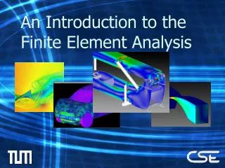
An Introduction to the Finite Element Analysis Presented by Niko Manopulo
Agenda PART I Introduction and Basic Concepts 1.0 Computational Methods 1.1 Idealization 1.2 Discretization 1.3 Solution 2.0 The Finite Elements Method 2.1 FEM Notation 2.2 Element Types 3.0 Mechanichal Approach 3.1 The Problem Setup 3.2 Strain Energy 3.3 External Energy 3.4 The Potential Energy Functional
Agenda PART II Mathematical Formulation 4.0 The Mathematics Behind the Method 4.1 Weighted Residual Methods 4.2 Approxiamting Functions 4.3 The Residual 4.4 Galerkin’s Method 4.5 The Weak Form 4.6 Solution Space 4.7 Linear System of Equations 4.8 Connection to the physical system
Agenda PART III Finite Element Discretization 5.0 Finite Element Discretization 4.1 The Trial Basis 4.2 Matrix Form of the Problem 4.3 Element Stiffness Matrix 4.4 Element Mass Matrix 4.5 External Work Integral 4.6 Assembling 4.7 Linear System of Equations 6.0 References 7.0 Question and Answers
PART I Introduction and Basic Concepts
1.1 Idealization • Mathematical Models • “A model is a symbolic device built to simulate and predict aspects of behavior of a system.” • Abstraction of physical reality • Implicit vs. Explicit Modelling • Implicit modelling consists of using existent pieces of abstraction and fitting them into the particular situation (e.g. Using general purpose FEM programs) • Explicit modelling consists of building the model from scratch
1.2 Dicretization • Finite Difference Discretization • The solution is discretized • Stability Problems • Loss of physical meaning • Finite Element Discretization • The problem is discretized • Physical meaning is conserved on elements • Interpretation and Control is easier
1.3 Solution • Linear System Solution Algorithms • Gaussian Elimination • Fast Fourier Transform • Relaxation Techniques • Error Estimation and Convergence Analysis
2.0 Finite Element Method • Two interpretations • Physical Interpretation: The continous physical model is divided into finite pieces called elements and laws of nature are applied on the generic element. The results are then recombined to represent the continuum. • Mathematical Interpretation: The differetional equation reppresenting the system is converted into a variational form, which is approximated by the linear combination of a finite set of trial functions.
2.1 FEM Notation Elements are defined by the following properties: • Dimensionality • Nodal Points • Geometry • Degrees of Freedom • Nodal Forces (Non homogeneous RHS of the DE)
3.0 Mechanical Approach • Simple mechanical problem • Introduction of basic mechanical concepts • Introduction of governing equations • Mechanical concepts used in mathematical derivation
3.2 Strain Energy • Hooke’s Law: where • Strain Energy Density:
3.2 Strain Energy (cont’d) • Integrating over the Volume of the Bar: • All quantities may depend on x.
3.3 External Energy • Due to applied external loads • The distributed load q(x) • The point end load P. This can be included in q. • External Energy:
3.4 The Total Potential Energy Functional • The unknown strain Function u is found by minimizing the TPE functional described below:
PART II Mathematical Formulation
4.0 Historical Background • Hrennikof and McHenry formulated a 2D structural problem as an assembly of bars and beams • Courant used a variational formulation to approximate PDE’s by linear interpolation over triangular elements • Turner wrote a seminal paper on how to solve one and two dimensional problems using structural elements or triangular and rectangular elements of continuum.
4.1 Weighted Residual Methods The class of differential equations containing also the one dimensional bar described above can be described as follows :
4.1 Weighted Residual Methods It follows that: Multiplying this by a weight function v and integrating over the whole domain we obtain: For the inner product to exist v must be “square integrable” Therefore: Equation (2) is called variational form
4.2 Approximating Function • We can replace uand vin the formula with their approximation function i.e. • The functionsfjandyj are of our choice and are meant to be suitable to the particular problem. For example the choice of sine and cosine functions satisfy boundary conditions hence it could be a good choice.
4.2 Approximating Function • U is called trial function and V is called test function • As the differential operator L[u] is second order • Therefore we can see U as element of a finite-diemnsional subspace of the infinite-dimensional function space C2(0,1) • The same way
4.3 The Residual • Replacing v and u with respectively V and U (2) becomes • r(x) is called the residual (as the name of the method suggests) • The vanishing inner product shows that the residual is orthogonal to all functions V in the test space.
4.3 The Residual • Substituting into and exchanging summations and integrals we obtain • As the inner product equation is satisfied for all choices of V in SN the above equation has to be valid for all choices of dj which implies that
4.4 Galerkin’s Method • One obvious choice of would be taking it equal to • This Choice leads to the Galerkin’s Method • This form of the problem is called the strong form of the problem. Because the so chosen test space has more continuity than necessary. • Therefore it is worthwile for this and other reasons to convert the problem into a more symmetrical form • This can be acheived by integrating by parts the initial strong form of the problem.
4.5 The Weak Form • Let us remember the initial form of the problem • Integrating by parts
4.5 The Weak Form • The problem can be rewritten as where • The integration by parts eliminated the second derivatives from the problem making it possible less continouity than the previous form. This is why this form is called weak form of the problem. • A(v,u)is called Strain Energy.
4.6 Solution Space • Now that derivative of v comes into the picture v needs to have more continoutiy than those in L2. As we want to keep symmetry its appropriate to choose functions that produce bounded values of • As p and z are necessarily smooth functions the following restriction is sufficient • Functions obeying this rule belong to the so called Sobolev Space and they are denoted by H1. We require v and u to satisfy boundary conditions so we denote the resulting space as
4.7 Linear System of Equations • The solution now takes the form • Substituting the approximate solutions obtained earlier in the more general WRM we obtain • More explicitly substituting U and V (remember we chose them to have the same base) and swapping summations and integrals we obtain
4.8 Connection to the Physical System Mechanical Formulation Mathematical Formulation
PART III Finite Element Discretization
5.0 Finite Element Discretization • Let us take the initial value problem with constant coefficients • As a first step let us divide the domain in N subintervals with the following mesh • Each subinterval is called finite element.
5.1 The Trial Basis • Next we select as a basis the so called “hat function”.
5.1 The Trial Basis • With the basis in the previous slide we construct our approximate solution U(x) • It is interesting to note that the coefficients correspond to the values of U at the interior nodes
5.1 The Trial Basis • The problem at this point can be easily solved using the previously derived Galerkin’s Method • A little more work is needed to convert this problem into matrix notation
5.2 Matrix Form of the Problem • Restricting U over the typical finite element we can write • Which in turn can be written as in the same way
5.2 Matrix Form of the Problem • Taking the derivative • Derivative of V is analogus
5.2 Matrix Form of the Problem • The variational formula can be elementwise defined as follows:
4.3 The Element Stiffnes Matrix • Substituting U,V,U’ and V’ into these formulae we obtain
4.4 The Element Mass Matrix • The same way
4.5 External Work Integral • The external work integral cannot be evaluated for every function q(x) • We can consider a linear interpolant of q(x) for simplicity. • Substituting and evaluating the integral Element load vector
4.6 Assembling • Now the task is to assemble the elements into the whole system in fact we have to sum each integral over all the elements • For doing so we can extend the dimension of each element matrix to N and then put the 2x2 matrix at the appropriate position inside it • With all matrices and vectors having the same dimension the summation looks like
4.6 Assembling • Doing the same for the Mass Matrix and for the Load Vector
4.7 Linear System of Equations • Substituting this Matrix form of the expressions in we obtain the following set of linear equations • This has to be satisfied for all choices of d therefore
References • Carlos Felippa http://caswww.colorado.edu/courses.d/IFEM.d/IFEM.Ch06.d/IFEM.Ch06.pdf • Joseph E Flaherty,Amos Eaton Professor http://www.cs.rpi.edu/~flaherje/FEM/fem1.ps • Gilbert Strang, George J. Fix An Analysis of the Finite Element Method Prentice-Hall,1973