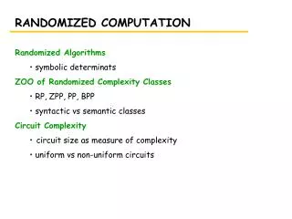
RANDOMIZED COMPUTATION

1. RANDOMIZED COMPUTATION • Randomized Algorithms • symbolic determinats • ZOO of Randomized Complexity Classes • RP, ZPP, PP, BPP • syntactic vs semantic classes • Circuit Complexity • circuit size as measure of complexity • uniform vs non-uniform circuits

2. SYMBOLIC DETERMINANTS • determinant of a matrix A: • det A = Sps(p)Pi=1n Ai,p(i) • where p goes over all permutations of n elements • s(p) = (-1)t(p) where t(p) is the number of transpositions of p • Determinants have many, many applications... • Symbolic matrix • the elements of the matrix are symbols, not numbers • symbols correspond to variables • Important question: Is the determinant of a given symbolic matrix identically equal to 0? • i.e. whatever values the variables take, the result is always 0? • det AG = 0 iff the bipartite graph G has perferct matching

3. SYMBOLIC DETERMINANTS • Computing symbolic determinants. • straightforward computing of the determinant from the definition? • exponential – all permutations of n elements, all possible variable values • Using Gaussian elimination • row operations do not change the determinant • once the matrix is reduced to triangular form, the determinant is the product of the diagonal • works well for a matrix with numbers – polynomial alg. • in symbolic matrices, the element sizes grow exponentially

4. SYMBOLIC DETERMINANTS • Lemma: Let p(x1, x2, …, xm) be a polynomial, not identically zero, in m variables, each of degree at most d, and let M>0 be an integer. Then the numnber of tuples (x1, x2, …, xm) {0,1,…, M-1}m such that p(x1, x2, …, xm)=0 is at most mdMm-1. • Note that for m=1, this says that a polynomial of degree d has at most d roots. • The proof is by induction on m (omitted). • This lemma gives the following idea for checking whether the given symbolic determinant is identically equal to 0: • choose m random integers i1, i2, …, im between 0 and M=2m • compute the determinant D in the matrix A(i1, i2, … im) using Gaussian elimination • if D 0 reply “The symbolic determinant is not identically 0” • else replay “The determinant is probably 0.”

5. SYMBOLIC DETERMINANTS • Note that if we give positive answer (the deterimnant is not identically 0), we are 100% of its correctness. • But there may be false negatives – we answer “determinant is probably 0” in some cases when the determinant is not identically 0 • What is the probability of false negatives? • mdMm-1/Mm • since d=1 and M=2m, we get ½ • How can we reduce the probability of false negatives? • increase M • repeat the experiment with new randomly generated values • the probability of false negatives can be brought down really fast • We got a Monte Carlo probabilistic algorithm

6. RANDOMIZED ATTACK AT SAT • Consider the following randomized algorithm for solving SAT: • Start with a random truth assignment T and repeat r times • if all clauses are satisfied, replay “formula is satisfiable” • otherwise pick an unsatisfied clause and a literal in that clause • flip the value of the corresponding variable • After r repetitions, return “formula is probably unsatisfiable” • Called random walk algorithm

7. RANDOMIZED ATTACK AT SAT • Can the random walk algorithm actually work? • i.e. after polynomial number of steps the probability of false negatives is less then ½? • Unfortunately, not (see Problem 11.5.6.) • However, it works well enough for 2SAT: • Theorem: A random walk algorithm with r=2n2 applied to a satisfiable instance of 2SAT with n variables will find a satisfying truth assignment with probability at least ½. • too bad we already know how to polynomially solve 2SAT

8. RANDOMIZED COMPLEXITY CLASSES • How to define a TM reflecting randomized algorithms? • no coin flipping is necessary • just different interpretation of what does it mean for the machine to accept the input • we can limit ourselves to precise TMs, in which each non-deterministic choice has exactly 2 branches • A polynomial Monte Carlo TM for a language L is a non-det TM standardized as above (i.e. each computation has length p(n) for each input of size n) such that for each input x the following is true: • if xL, then at least half of computations halt in “yes” state • if xL then all computations halt in “no” state

9. RANDOMIZED COMPLEXITY CLASSES • RP (randomized polynomial time) – the class of languages recognized by polynomial Monte Carlo TMs. • the 1/2 probability of false negatives in the definition is not crucial, it can be replaced by any number less the 1-e for some fixed e • just repeat the random experiment enough times, until (1-e)k<1/2 • Where does RP lie with respect to the classes we have seen so far? • somewhere between P and NP

10. SYNTACTIC vs SEMANTIC CLASSES • For classes like P and NP and other time/space bounded classes, we had a mechanical way to ensure that the machine is in that class • for every machine in that class there is an equivalent one where we added a time or space yardstick • we call these classes syntactic complexity classes • But with machines from RP, the requirement for being in class is not time/space bound, but peculiar acceptance behavior: • either accept by majority, or reject unanimously • there is no easy way to standardize/tell whether a machine is in RP or not • RP is a semantic class • other examples include NP  coNP and TFNP

11. SYNTACTIC vs SEMANTIC CLASSES • Syntactic classes have a “standard” complete language: • {(M,x): M  M and M(x) = “yes”}, where M is the class of all machines that define the class, appropriately standardized. • For semantic classes, the “standard” complete language is usually undecidable • semantic classes do not have complete problems

12. THE CLASS ZPP • Is RP closed under complement? • the definition is highly asymmetric, so with high probability no • What about the class RP  coRP? • for RP, there are no false positives • but if we keep getting negative answers, we don’t know for sure whether the answer is truly “no” • for coRP, there are no false negatives • similarly for “yes” in coRP • for both, the longer we re-run the algorithm, the less the chance of error, but we can never be 100% sure

13. THE CLASS ZPP • If a language is in RP  coRP, there are two algorithms, one without false positives, another without false negatives • if we run both algorithms independently and repeatedly, we will eventually get either “yes” from the first one, or “no” from the second one • at that moment, we are 100% sure of the correctness • the only problem is that there is non-zero (but diminishingly small) probability of long run • such algorithms are called Las Vegas probabilistic algorithms • The class RP  coRP is called ZPP (zero probability of error)

14. THE CLASS PP • Consider the MAJSAT problem: Given a Boolean expression, is it true that the majority of the 2n truth assignments satisfy it? • it is not clear whether MAJSAT is even in NP • the certificate is huge • The natural class for MAJSAT to lie in is the class PP: • A language is in the class PP iff there is nondeterministic polynomially bounded TM M(standardized as above) such that for all inputs x, xL iff more then half of computations M on input x end up accepting. (We say that M decides by “majority”.)

15. THE CLASS PP • Is PP semantic or syntactic class? • any standardized TM can be used to define a language from PP • so PP is syntactic • Theorem: MAJSAT is PP complete • Theorem: NP  PP • for any language LNP, construct a TM M that accepts L by majority: • split initially into two subtrees, the left one accepts all, the right one is the original • the input is accepted by majority iff there is accepting execution in the right subtree • Theorem:PP is closed under complement (almost symmetric definition)

16. THE CLASS BPP • The classes P, RP and ZPP correspond to plausible computation • The class PP does not • it is a natural way to capture certain computational problems • but does not have realistic computational content • i.e. similar to NP • Where is the problem? • acceptance by majority is too “fragile” • there is a very small difference between accepting and rejecting in PP, and there is no way to exploit this difference • i.e. like trying to detect biased coin which is arbitrarily close to ½ - might need exponential number of tries to see the bias

17. THE CLASS BPP • Idea: Separate the accepting and rejecting states, so the difference can be efficiently computationally observed. • Definition: The class BPP contains all languages L for which there is a nondeterministic polynomially bounded TM M (standardized, as usual) such that • if xL then at least ¾ of the computations of M on input x accept • if x L then at least ¾ of the computations reject • Note: ¾ is not necessary, any number strictly between ½ and 1 will do • BPP is perhaps the strongest notion of plausible computation.

18. THE CLASS BPP • Obviously, RP  BPP  PP • the probability of false positives/negatives in BPP must be at most ¼. RP has no false positives and the probability of false negatives is at most ½, so run an RP algorithm twice to reduce that probability to ¼. • a machine that decides by clear majority (3/4) clearly also decides by simple majority • Is BPP  NP? • open problem • Is BPP closed under complement? • yes, symmetric definition • Is BPP syntactic or semantic class? • semantic, no way to check whether the acceptance conditions are satisfied

19. PP coNP NP coRP RP BPP P THE ZOO ZPP

20. CIRCUIT COMPLEXITY • Can boolean circuits be used to accept languages? • boolean circuits can compute any boolean function on n variables • so, for a given language L, there exists a boolean circuit that accepts/rejects all words of length n, depending on whether they are in L or not • but L contains words of different lenghts • we need a family of circuits C = (C0, C1, …), where Cn has n input variables • Definition:Size of a circuit – number of gates. A language L has polynomial circuits if there is a familiy of circuits C=(C0, C1, …) such that: • the size of Cn is at most p(n) for some fixed polynomial p • xL iff the output of C|x| on x is true

21. REACHABILITY HAS POLYNOMIAL CIRCUITS • We have essentially seen the proof when we reduced REACHABILITY to CIRCUIT VALUE: • two kinds of gates • gi,j,k ~ there is a path from i to j not using intermediate nodes higher then k • hi,j,k ~ there is a path from i to j not using intermediate nodes higher then k, but using k as intermediate node • gi,j,0 are the input gates • gi,j,0 is true iff i=j or (i,j) is an edge in G • hi,j,k is an and gate with inputs from gi,k,k-1 and gk,j,k-1 • gi,j,k is an or gate with inputs from gi,j,k-1 and hi,j,k,j,k-1 • g1,n,n is the output gate

22. P vs POLYNOMIAL CIRCUITS • Note that the above circuits is for graphs of n vertices. • A family of such circuits is needed for the REACHABILITY problem. • Theorem: All languages in P have polynomial circuits. • Again, we have already seen the proof before • when we proved that CIRCUIT VALUE is P-complete, we constructed a circuit essentially evaluating the computation of the polynomially boundedTM (the computational table technique) • the circuit was of size O(p(|x|)2)for input of length x • the only modification is changing the input gates from constants to variables

23. P vs POLYNOMIAL CIRCUITS • OK, so all languages in P have polynomial circuits. • Are all languages with polynomial circuits in P? • Theorem: There are undecidable languages that have polynomial circuits. • let L be any undecidable language in alphabet {0,1}, and let U be the language {1n:the binary expansion of n is in L} • U is undecidable • can you construct a polynomially bounded family of circuits recognizing U? • for each 1n U, Cn consists of AND gates of all its inputs • if 1n U, Cn has only input gates and one false output gate

24. P vs POLYNOMIAL CIRCUITS • So, undecidable languages might have polynomial circuits… • Where is the problem? • How to constuct the family of circuits accepting U? • you have to first solve the problem of recognizing L • i.e. to solve an undecidable problem! • not a very practical proposition • Definition: A family of circuits C=(C0, C1, …) is said to be uniform, if there is a log-space bounded TM M which on input 1n outputs Cn • A language L has uniformly polynomial circuits if there is a uniform family of polynomial circuits that decides L.

25. P vs POLYNOMIAL CIRCUITS • Theorem: A language L has uniformly polynomial circuits if and only if L  P. • we have already seen the  direction (computation table method), as the construction can be done in log space • : if L has uniformly polynomial circuits, then on input x we can construct C|x| in log(|x|) space (and therefore in time polynomial in |x|) and then evaluate C|x| in time polynomial in |x|

26. CIRCUITS and P vs NP • Conjecture A: NP-complete problems have no uniformly polynomial circuits. • Conjecture B: NP-complete problems have no polynomial circuits, uniform or not. • proving any of those conjecture would prove P  NP • so people are trying to find an NP-complete problem that has no polynomial circuits

27. BPP and Circuits • Theorem: All languages in BPP have polynomial circuits. • Proof: Let LBPP, i.e. there is a non-det TM M that decides by clear majority. We show that L has a polynomial family of circuits (C0, C1, …) by showing how to construct Cn for each n. • if our construction was simple and explicit, that would actually mean that BPP=P • but there is a non-constructive step in the construction

28. BPP and Circuits • Let An=(a1, a2, …, am) be a sequence of binary strings, each of length p(n), and m=12(n+1). • each ai represents a sequence of choices of M in a computation of length p(n) • Cn on input x of length n simulates M with each sequence of choices in An and then takes the majority of the outcomes • Cn is of polynomial size: O(m x p(n)2) • using the computational table method • But why would Cn produce correct result? • An does not contain all 2p(n) possible choices, only 12(n+1)

29. BPP and Circuits • Claim: For all n > 0 there is a set An of m=12(n+1) binary strings such that for all inputs x with |x|=n fewer then half of the choices are bad. • Consider a sequence An of m bit strings of length p(n) selected at random by independent sampling of {0,1}p(n). • What is the probability that for each x {0,1}n more then half of choices in An are correct? • We show that this probability is at least ½ • for each fixed x, at most quarter of computations are bad (from BPP definition) • by Chernoff bound the probability that the number of bad strings is m/2 or more for this fixed x is at most e-m/12<1/2n+1

30. BPP and Circuits The probability that a random selection of An is bad for fixed x is at most 1/2n+1 There are 2p(n)12(n+1) possible sequences An, and for each x{0,1}n at most 1/2n+1 of them is bad. Therefore, altogether there are at most 2n2p(n)12(n+1)/2n+1 =2p(n)12(n+1)/2 bad sequences, i.e. at least half of the possible sequences are good. Note that we did not specify how to find a good one, but we know that there is such a good An, in fact there are plenty of them.