Microbial Genomes
Microbial Genomes. 1) Methods for Studying Microbial Genomes 2) Analysis and Interpretation of Whole Genome Sequences. Methods for Studying Microbial Genomes. Why study genomes? History of genome sequencing Methods, Principles & Approaches. Why study microbial genomes?.

Microbial Genomes
E N D
Presentation Transcript
Microbial Genomes • 1) Methods for Studying Microbial Genomes • 2) Analysis and Interpretation of Whole Genome Sequences
Methods for Studying Microbial Genomes Why study genomes? History of genome sequencing Methods, Principles & Approaches
Why study microbial genomes? • until whole genome analysis became viable, life sciences have been based on a reductionist principle – dissecting cell and systems into fundamental components for further study • studies on whole genomes and whole genome sequences in particular give us a complete genomic blueprint for an organism • we can now begin to examine how all of these parts operate cooperatively to influence the activities and behavior of an entire organism – a complete understanding of the biology of an organism • microbes provide an excellent starting point for studies of this type as they have a relatively simple genomic structure compared to higher, multicellular organisms • studies on microbial genomes may provide crucial starting points for the understanding of the genomics of higher organisms
Why study microbial genomes? • analysis of whole microbial genomes also provides insight into microbial evolution and diversity beyond single protein or gene phylogenies • in practical terms analysis of whole microbial genomes is also a powerful tool in identifying new applications in for biotechnology and new approaches to the treatment and control of pathogenic organisms
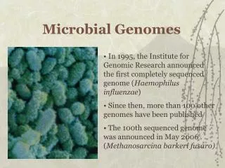
History of microbial genome sequencing • 1977 - first complete genome to be sequenced was bacteriophage X174 - 5386 bp • first genome to be sequenced using random DNA fragments - Bacteriophage - 48502 bp • 1986 - mitochondrial (187 kb) and chloroplast (121 kb) genomes of Marchantia polymorpha sequenced • early 90’s - cytomegalovirus (229 kb) and Vaccinia (192 kb) genomes sequenced • 1995 - first complete genome sequence from a free living organism - Haemophilus influenzae (1.83 Mb) • late 1990’s - many additional microbial genomes sequenced including Archaea (Methanococcus jannaschii - 1996) and Eukaryotes (Saccharomyces cerevisiae - 1996)
Microbial genomes sequenced to date • currently there are 32 complete, published microbial genomes – 25 domain Bacteria, 5 Domain Archaea, 1 domain Eukarya (www.tigr.org) • around 130 additional microbial genome and chromosome sequencing projects underway
Laboratory tools for studying whole genomes • conventional techniques for analysing DNA are designed for the analysis of small regions of whole genomes such as individual genes or operons • many of the techniques used to study whole genomes are conventional molecular biology techniques adapted to operate effectively with DNA in a much larger size range
Pulsed Field Gel Electrophoresis • agarose gel electrophoresis is a fundamental technique in molecular biology but is generally unable to resolve fragments greater than 20 kilobases in size (whole microbial genomes are usually greater than 1000 kilobases in size) • PFGE (pulsed field gel electrophoresis) is a adaptation of conventional agarose gel electrophoresis that allows extremely large DNA fragments to be resolved (up to megabase size fragments) • essential technique for estimating the sizes of whole genomes/chromosomes prior to sequencing and is necessary for preparing large DNA fragments for large insert DNA cloning and analysis of subsequent clones • also a commonly used and extremely powerful tool for genotyping and epidemiology studies for pathogenic microorganisms
Principle of PFGE • two factors influence DNA migration rates through conventional gels • - charge differences between DNA fragments • - ‘molecular sieve’ effect of DNA pores • DNA fragments normally travel through agarose pores as spherical coils, fragments greater than 20 kb in size form extended coils and therefore are not subjected to the molecular sieve effect • the charge effect is countered by the proportionally increased friction applied to the molecules and therefore fragments greater than 20 kb do not resolve • PFGE works by periodically altering the electric field orientation • the large extended coil DNA fragments are forced to change orientation and size dependent separation is re-established because the time taken for the DNA to reorient is size dependent
Principle of PFGE • the most important factor in PFGE resolution is switching time, longer switching times generally lead to increased size of DNA fragments which can be resolved • switching times are optimised for the expected size of the DNA being run on the PFGE gel • switch time ramping increases the region of the gel in which DNA separation is linear with respect to size • a number of different apparatus have been developed in order to generate this switching in electric fields however most commonly used in modern laboratories are FIGE (Field Inversion Gel Electrophoresis) and CHEF (Contour-Clamped Homogenous Electrophoresis)
CHEF Switch Time Electric Field 1 Electric Field 2 - - - - - - - - + + + + + + + +
Preparation of DNA for PFGE • ideally a genomic DNA preparation that contains a high proportion of completely or almost completely intact genome copies would be suitable for PFGE • conventional means of DNA preparation are unsuitable for PFGE as mechanical shearing and low-level nuclease activity will result in fragmented DNA with an average size much smaller than an entire microbial genome (usually less than 200 kb in size) • the solution to this is to prepare genomic DNA from whole cells in a semisolid matrix (ie. agarose) that eliminates mechanical shearing • a very high concentration of EDTA is also used at all times in order to eliminate all nuclease activity
Preparation of DNA for PFGE • Procedure – • 1) intact cells are mixed with molten LMT agarose and set in a mold forming agarose ‘plugs’ • 2) enzymes and detergents diffuse into the plugs and lyse cells • 3) proteinase K diffuses into plugs and digests proteins • 4) if necessary restriction digests are performed in plugs (extensive washing or PMSF treatment is required to remove proteinase K activity) • 5) plugs are loaded directly onto PFGE and run
Preparation of DNA for PFGE • for restriction digests, conventional enzymes are unsuitable as they cut frequently on an entire genome sequence producing DNA fragments that are far too small • ‘rare cutter’ restriction endonucleases cut genomic DNA with far less frequency than conventional restriction enzymes such as HindIII, BamHI etc. • many rare cutter RE’s have 6-bp (or longer) recognition sites eg. NotI GCGGCCGC • in many cases the frequency of cutting is highly species dependent eg. BamHI will cut far less frequently on a low GC% genome when compared to a intermediate or high GC content genome • suitable rare cutter enzymes therefore have to be determined experimentally for each new species being studied
Large insert cloning vectors – BAC’s and PAC’s • DNA cloning is another technique fundamental to molecular biology that requires adaptation in order to be useful in studying DNA at a whole genome scale • conventional plasmid derived cloning vectors are only able to reliably maintain inserts less than 20 kb in size • there are a number of approaches to generating clones with inserts in an intermediate size range (20 – 80 kB) such as cosmids, etc. • the most commonly used vectors for cloning extremely large DNA inserts are BAC’s (Bacterial Artificial Chromosomes) and PAC’s (P1-derived Artificial Chromosomes) • both BAC and PAC vectors are plasmid derived vectors distinguished from conventional vectors by extremely tightly controlled low copy numbers
Large insert cloning vectors – BAC’s and PAC’s • these very low copy numbers help to limit the strain on host cellular resources generated by very large DNA inserts thus eliminating the rejection of large insert clones • low copy numbers also help to limit recombination events with host genomic DNA • BAC and PAC vectors both utilise E. coli as the host organism • BAC vectors are based on the E. coli single copy F-factor plasmid – the F-factor origin of replication is very tightly controlled • PAC vectors are based on an identical principle but instead use a single copy origin of replication derived from P1 phage • PAC vectors also contain a pUC19 cassette for improved vector purification
Approaches to whole microbial genome sequencing • aim of microbial genome sequencing projects is to construct, from 500 – 800 bp sequencing reads containing about 1% mistakes, a genome sequence of several megabases with an error rate lower than 1 per 10000 nucleotides • with improving software, decreasing computation costs and advancements in automated DNA sequencing, an entire microbial genome project can be completed in a small laboratory in 1-2 years • there are two main approaches to sequencing microbial genomes – the ordered clone approach and direct shotgun sequencing • both require both large and small insert genomic DNA libraries in order to be effective
Ordered Clone Approach • essentially this technique involves constructing a map of overlapping large insert clones covering the whole genome and then completely sequencing the minimum subset of these ordered clones • there are a number of methods used to order clones including restriction fingerprinting and hybridisation mapping • once an ordered large insert clone set is identified, a whole genome sequence is determined by either shotgun or partial primer walk sequencing of each insert • the ordered clone approach to DNA sequencing requires a large amount of characterisation prior to actual DNA sequencing and is therefore a relatively time consuming approach, however, it may be cheaper than shotgun sequencing an entire genome as less redundant sequencing is required • with rapid decreases in costs for computing power and sequencing this method is no longer considered viable for small (< 5 Mb) genomes
Large DNA fragment Digest and subclone Whole Genome Randomly sequence fragments Fill gaps Repeat for entire genome map
Random sequencing (shotgun) approach • this is the currently the most commonly used strategy for microbial whole genome sequencing • sequences from both ends of a large number of small and large insert clones are generated and overlapping sequences joined together to form a ‘contig’ of the whole genome sequence (whole inserts not sequenced) • although this requires enormous amounts of DNA sequencing (often up to 10x genome coverage) and computational power for sequence assembly, it is a relatively rapid approach to whole genome sequencing • the first 90 – 95% of the genome sequence is relatively easy to generate by shotgun sequencing resulting in several hundred discrete contigs • filling the gaps to produce a single contig is the most difficult and time consuming phase of this process
Shear and subclone Whole Genome Randomly sequence fragments Fill gaps
Random sequencing (shotgun) approach • There are a number of steps in the process - • 1) Random large and small insert library construction • 2) High throughput DNA sequencing • 3) Sequence assembly • 4) Ordering of contigs • 5) Primer walking to complete sequence • 6) Annotation
Library construction • Both conventional and large insert genomic DNA libraries should be constructed • the small insert library will be used for the bulk of the sequencing in order to generate suitable coverage of the complete genome • the large insert library (BAC, PAC, cosmid etc.) will be used as a ‘scaffold’ during the sequence closure phase • it is crucial to ensure that both libraries are as random as possible - mechanical shearing is often used to generate small DNA fragments • it is also important that each clone contains only one DNA fragment and as such specialised methods for library construction must be used
DNA Sequencing • DNA sequences are generated using vector primers for both ends of inserts • at least 6X coverage of the genome is required although 9 to 10X coverage is often generated
Sequence assembly and gap closure • 4 major steps in sequence assembly and gap closure - • 1) random sequences initially interpreted using highly accurate base calling software and assembled to generate primary contigs using software such as PHRAPP • 2) computational and experimental techniques used to identify linking clones and order primary contigs • 3) primer walk sequencing of linking clones and PCR products to fill sequence gaps between contigs • 4) confirmation of contig order by PCR
Linking Clones • one of the most effective means of contig ordering and gap filling is linking clones • linking clones are those whose terminal sequences (from either end of the insert) belong to different contigs • if the orientation of the sequences and the distance to the end of the contig are compatible with with the size of the insert, the two contigs are likely to be linked • the larger the insert the more likely a clone will be a linking clone • this is why random sequencing is also performed on large insert clones - they are far more likely to form linking clones
Contig 1 Contig 2 Gap Random Sequencing Random Sequencing
Large Insert Linking Clone Contig 1 Contig 2 • Once all possible linking clones are identified - • gaps are classified into two categories - those with linking clones (template available for sequencing) and physical gaps without linking clones ( no DNA template for the region) • for those gaps with suitable linking clones, the gaps confirmed by PCR and closed by primer walk sequencing REV FWD
Large insert Linking Clone Contig 1 Contig 2 REV FWD Primer Walking
Physical Gaps • Contigs separated with physical gaps (no linking clones) are usually spanned by PCR on genomic DNA using primers from each end of the contigs • the PCR products can then be sequenced to close the gaps • without linking clones other techniques to order contigs must be used in order to guide the selection of PCR products
For those contigs without linking clones, how do you fill the gaps? Linking clone Supercontig 1 Supercontig 2 Supercontig 3
Physical Gaps • contigs can be ordered by - • peptide linking - contig ends having regions with homology to the same gene (or operon / gene cluster) • southern hybridisation of labelled contig terminal oligonucleotides against large restriction fragments
Linked by Southern Hybridisation Contig 2 PCR Product Contig 6 FWD REV Primer Walking
Gapped Microbial Genomes • considering the cost and difficulty in filling gaps between contigs some interest has been generated by the analysis of gapped microbial genomes • each gap is usually very small on average (approximately 75 bp for a 3.2x coverage library) • increasing bioinformatic resources available mean that these gaps have little influence on functional reconstruction • eg. Thiobacillus ferroxidans - all assigned amino acid biosynthesis genes (140 in total) identified from a gapped genome of 1912 contigs • error rates tend to be relatively high compared to genome sequences with greater coverage
Example - Haemophilus influenzae • first complete genome sequence of a free living organism (1995) • important pathogen • genome is around 1.83 megabases in size • random sequencing was done for both small insert and large insert (lambda) libraries • sequencing reactions performed by eight individuals using fourteen ABI 377 DNA sequencers per day over a three month period • in total around 33000 sequencing reactions were performed on 20000 templates • plasmid extraction performed in a 96 well format • 11 mb of sequence was intially used to generate 140 contigs • gaps were closed by lambda linking clones (23), peptide links (2), Southern analysis (37) and PCR (42)
Annotation of Genome Sequences • a microbial genome sequence alone is only raw data – it needs to be interpreted in order to be of any scientific significance • the process of predicting the location and function of all possible coding sequences (genes) in a genome sequence is known as annotation • although an annotated genome sequence provides a large amount of important information it is still merely a starting point for completely characterising an organism • Genome Databases: • Listing of genomes: Genomes online database (GOLD) • Comprenehsive Genome Databases : GenBank, EMBL, DDBJ, JGI, TIGR, HAMAP, IMG, PEDANT (curation problematic, special tools for exploring / comparing / aligning genomes) • Taxon specific Genome Database: EcoCyc (literature derived annotations)
Genome Annotation The process after sequencing has been completed. Use of many different tools required: Bioinformatics Databases Literature Sequence Experimental
Sequence Gene prediction Proteins Similarity searches against reference databases Calculations & predictions (MW , structure, location etc) Annotated Proteins Pathway prediction Manual editing Annotated Proteins & pathways Data visualization Pipeline for genome annotation
Identifying ORF’s • most genomes will contain genes with very little or no homology to known genes of other organisms • for this reason all of the possible ORF’s need to be identified without relying totally on homology • most efficient means for identifying potential genes in genome sequences is a three step process • 1) submit entire sequence as a 6-frame translation for BLAST analysis in order to identify some protein coding regions on the basis of high levels of homology • 2) use these initial coding regions to determine the sequence characteristics (GC content, codon bias etc.) that distinguish coding and non-coding regions of the genome (‘training’ the software
Identifying ORF’s • 3) reanalyse the genome sequence using this data (plus potential ribosome binding sequences) in order to identify all the potential genes • using this process it has been experimentally shown that around 94% of genes can be accurately predicted • algorithms are also available to identify ORF’s without using the training procedure with only slightly reduced accuracy • GLIMMER is a software for gene prediction and used by: • BASYS- http://wishart.biology.ualberta.ca/basys/cgi/submit.pl • JCVI (formerly TIGR)- http://www.tigr.org/ • SABIA- http://www.sabia.lncc.br/
Assigning function to ORF’s • in order to assign function, all predicted ORF’s are translated to amino acid sequence and analysed by homology searches against sequence databases (usually Genbank) • for each ORF there are three possible results - • i) clear sequence homology indicating function • ii) blocks of homology to defined functional motifs • - these should be confirmed experimentally • iii) no significant homology or homology to proteins of unknown function
ORF’s of unidentified function • in most genome sequences many of the ORF’s identified cannot be assigned a specific function based on homology • although the figure varies, usually between 40 and 50% of ORF’s fall into this category • clearly this represents a significant gap in our knowledge of microbial metabolism • these ORF’s can be further divided into two categories – • i) conserved hypothetical proteins – ORF’s with no homology to proteins of known function but with significant homology to unidentified ORF’s of other species • these ORF’s are therefore functionally conserved across numerous species and may represent important components of central metabolism that have not yet been identified
ORF’s of unidentified function • the more universal the distribution of these ORF’s the more likely they have a fundamental role in metabolism • ii) ORF’s without homologues – these are ORF’s that have no homology to any known sequences – these may represent genes encoding proteins related to more specific organism adaptations • eg. Deinococcus radiodurans is a radiation resistant organism that contains many ORF’s without homologues – many of these are thought to be involved in specialised processes of DNA repair
ORF identification and new amino acids In addition to the 20 amino acids, two new but rare amino acids have now been identified: • 21st selenocystine (Sec) • 22nd pyrolysin (Pyl) The Sec and Pyl containing proteins are predominantly found in members of class δ-proteobacteria, phylum Proteobacteria. Metagenome analysis of the uncultured δ-proteobacteria of the gutless & mouthless worm, Olavius algarvensi, contains the highest proportion of Sec & Pyl containing proteins to date suggesting that symbiosis promotes Sec & Pyl genetic code Olavius algarvensi, also contains the most wide use of the genetic code- 63 out of the 64 possible codons Sec: • 99 genes, cluster into 30 protein families • present in domains Bacteria, Archaea & Eucarya. • Sec coded by UGA (UGA also acts as a stop codon)