LIS 570
LIS 570. Session 7.1 Bivariate Data Analysis. Objectives. Reinforce concept of standard error and the standard normal distribution (basis of confidence level and confidence interval) Understand different approaches to the analysis of bivariate data Gain confidence in use of SPSS. Agenda.

LIS 570
E N D
Presentation Transcript
LIS 570 Session 7.1 Bivariate Data Analysis
Objectives • Reinforce concept of standard error and the standard normal distribution (basis of confidence level and confidence interval) • Understand different approaches to the analysis of bivariate data • Gain confidence in use of SPSS
Agenda • Review Central Limit Theorem • Visualization of “confidence interval” and “confidence level” • Overview of bivariate analysis approaches • Exploratory data analysis using SPSS
Shapes of distribution Normal distribution:symmetrical Bell-shapedcurve symmetrical asymmetrical Negatively skewed:tail on the left, cluster towards high-end of the variable Positively skewed:tail on the right, cluster towards low end of the variable Bimodality: A double peak
Central Limit Theorem The CLT states: regardless of the shape of the population distribution, as the number of samples (N) becomes very large (approaches infinity) the distribution of the sample mean ( m ) is normally distributed, with a mean of µ and standard deviation of σ/(√N).
Standard Error of the Mean Standard error of the mean (Sm) Sm = N • Standard error is inversely related to square root of sample size • To reduce standard error, increase sample size • Standard error is directly related to standard deviation • When N = 1, standard error is equal to standard deviation S Standard deviation S Total number in the sample
Inferential statistics - univariate analysis Interval estimates and interval variables • Estimation of sample mean accuracy—based on random sampling and probability theory Standardize the sample mean to estimate population mean: t = sample mean – population mean estimated SE Population mean = sample mean + t * (estimated SE)
Exercise—sampling distribution • Coin tossing • Probability of head or tails—50% • Each of you is a “sample” for this activity. • Flip the coin 9 times, count the # of times you get a “head”. Live demo: http://www.ruf.rice.edu/~lane/stat_sim/sampling_dist/index.html
Standard Error(for nominal & ordinal data) Variable must have only two categories (could combine categories to achieve this) SB = PQ N P = the % in one category of the variable Q = the % in the other category of the variable Total number in the sample Standard error for binominal distribution
Choosing the Statistical Technique* Specific research question or hypothesis Determine # of variables in question Univariate analysis Bivariate analysis Multivariate analysis Determine level of measurement of variables Choose univariate method of analysis * Source: De Vaus, D.A. (1991) Surveys in Social Research. Third edition. North Sydney, Australia: Allen & Unwin Pty Ltd., p133 Choose relevantdescriptive statistics Choose relevantinferential statistics
Association • Example: gender and voting • Are gender and party supported associated (related)? • Are gender and party supported independent (unrelated)? • Are women more likely than men to vote republican?Are men more likely to vote democrat?
Association Association in bivariate data means that certain values of one variable tend to occur more often with some values of the second variable than with other variables of that variable (Moore p.242) Correlation Coefficient Cross Tabulation
Cross Tabulation Tables • Designate the X variable and the Y variable • Place the values of X across the table • Draw a column for each X value • Place the values of Y down the table • Draw a row for each Y value • Insert frequencies into each CELL • Compute totals (MARGINALS) for each column and row
Determining if a Relationship Exists • Compute percentages for each value of X (down each column) • Base = marginal for each column • Read the table by comparing values of X for each value of Y • Read table across each row • Terminology • strong/ weak; positive/ negative; linear/ curvilinear
Cross tabulation tables Occupation Calculate percent Vote Read Table (De Vaus pp 158-160)
Cross tabulation • Use column percentages and compare these across the table • Where there is a difference this indicates some association
Describing association Strong - Weak Direction Strength Positive - Negative Nature Linear - Curvilinear
Describing association Two variables are positively associated when larger values of one tend to be accompanied by larger values of the other The variables are negatively associated when larger values of one tend to be accompanied by smaller values of the other (Moore, p. 254)
Describing association Scattergram or scatterplot Graph that can be used to show how two interval level variables are related to one another Y Y Variable A weight X X Age Variable B
Description of Scattergrams • Strength of Relationship • Strong • Moderate • Low • Linearity of Relationship • Linear • Curvilinear • Direction • Positive • Negative
Description of scatterplots Y Y X X Strength and direction Y Y X X
Description of scatterplots Y Y Nature X X Strength and direction Y Y X X
Correlation • Correlation coefficient—number used to describe the strength and direction of association between variables • Very strong = .80 through 1 • Moderately strong = .60 through .79 • Moderate = .50 through .59 • Moderately weak = .30 through .49 • Very weak to no relationship 0 to .29 -1.00 Perfect Negative Correlation 0.00 No relationship 1.00 Perfect Positive Correlation
Correlation Coefficients • Nominal • Phi • Cramer’s V • Ordinal (linear) • Gamma • Nominal and Interval • Eta http://www.nyu.edu/its/socsci/Docs/correlate.html
Correlation: Pearson’s r • Interval and/or ratio variables • Pearson product moment coefficient (r) • two interval variables, normally distributed • assumes a linear relationship • Can be any number from • 0 to -1 : 0 to 1 (+1) • Sign (+ or -) shows direction • Number shows strength • Linearity cannot be determined from the coefficient e.g.: r = .8913
Summary • Bivariate analysis • crosstabulation • X - columns • Y - rows • calculate percentages for columns • read percentages across the rows to observe association • Correlation and scattergram: describe strength and direction of association