Data Mining and Data Warehousing, many-to-many Relationships, applications
460 likes | 769 Views
Data Mining and Data Warehousing, many-to-many Relationships, applications. William Perrizo Dept of Computer Science North Dakota State Univ. Why Mining Data?. Parkinson’s Law (for data) Data expands to fill available storage (and then some) Disk-storage version of Moore’s law

Data Mining and Data Warehousing, many-to-many Relationships, applications
E N D
Presentation Transcript
Data Mining and Data Warehousing, many-to-many Relationships, applications William Perrizo Dept of Computer Science North Dakota State Univ.
Why Mining Data? • Parkinson’s Law (for data) Data expands to fill available storage (and then some) • Disk-storage version of Moore’s law Capacity 2 t / 9 months • Available storage doubles every 9 months!
Another More’s Law: More is Less The more volume, the less information. (AKA: Shannon’s Canon) A simple illustration: Which phone book is more helpful? BOOK-1BOOK-2 Name NumberName Number Smith 234-9816 Smith 234-9816 Jones 231-7237 Smith 231-7237 Jones 234-9816 Jones 231-7237
Awash with data! • US EROS Data Center archives Earth Observing System (EOS) remotely sensed images (RSI), satellite and aerial photo data (10 petabytes by 2005 ~ 1016 B). • National Virtual Observatory (aggregated astronomical data) (10 exabytes by 2010 ~ 1019 B?). • Sensor networks (Micro and Nano -sensor networks) (10 zettabytes by 2015 ~ 1022 B?). • WWW will continue to grow (and other text collections) (10 yottabytes by 2020 ~ 1025 B?). • Micro-arrays, gene-chips and genome sequence data (10 gazillobytes by 20?0 ~ 1028 B?). Useful information must be teased out of these large volumes of data.That’s data mining. Correct Name?
TIFF image Yield Map EOS Data Mining example This dataset is a 320 row and 320 column (102,400 pixels) spatial file with 5 feature attributes (B,G,R,NIR,Y). The (B,G,R,NIR) features are in the TIFF image and the Y (crop yield) feature is color coded in the Yield Map (blue=low; red=high) What is the relationship between the color intensities and yield? We can hypothsize: hi_greenandlow_red hi_yield which, while not a simply SQL query result, is not surprising. Data Mining is more than just confirming hypotheses The stronger rule, hi_NIR and low_red hi_yield is not an SQL result and is surprising. Data Mining includes suggesting new hypotheses.
Another Precision Agriculture Example Grasshopper Infestation Prediction • Grasshopper caused significant economic loss each year. • Early infestation prediction is key to damage control. Association rule mining on remotely sensed imagery holds significant promise to achieve early detection. Can initial infestation be determined from RGB bands???
Gene1 Gene3 Gene5 Gene9 Gene6 Gene8 Gene Regulation Pathway Discovery • Results of clustering may indicate, for instance, that nine genes are involved in a pathway. • High confident rule mining on that cluster may discover the relationships among the genes in which the expression of one gene (e.g., Gene2) is regulated by others. Other genes (e.g., Gene4 and Gene7) may not be directly involved in regulating Gene2 and can therefore be excluded (more later). Gene1 Gene2, Gene3 Gene4, Gene 5, Gene6 Gene7, Gene8 Gene9 Clustering ARM Gene4 Gene7 Gene2
Sensor Network Data Mining • Micro, even Nano sensor blocks are being developed • For sensing • Bio agents • Chemical agents • Movements • Coatings deterioration • etc. • There will be billions, even trillions of individual sensors creating mountains of data. • The data must be mined for it’s meaning. • Other data requiring mining: • shopping market basket analysis (Walmart) • Keywords in text (e.g., WWW) • Properties of proteins • Stock market prediction • Astronomical data • UNIFIED BASES OF ALL THIS DATA??
Data Mining? Querying asks specific questions and expect specific answers. Data Mininggoes into the MOUNTAIN of DATA, and returns with information gems (rules?) But also, some fool’s gold? Relevance and interestingness analysis, serves as an assay (help pick out the valuable information gems).
Fractals, … Standard querying Searching and Aggregating Data Prospecting Machine Learning Data Mining Association Rule Mining OLAP (rollup, drilldown, slice/dice.. Supervised Learning – Classificatior Regression SQL SELECT FROM WHERE Complex queries (nested, EXISTS..) FUZZY query, Search engines, BLAST searches Unsupervised Learning - Clustering Data Mining versus Querying There is a whole spectrum of techniques to get information from data: On the Query Processing end, much work is yet to be done(D. DeWitt, ACM SIGMOD’02). On the Data Mining end, the surface has barely beenscratched. But even those scratches had a great impact – becoming the biggest corporation in the world and filing for bankruptcy Walmart vs.KMart
Data Mining Knowledge Pattern Evaluation • Data mining: the core of the knowledge discovery process. Data Mining OLAP Classification Clustering ARM Task-relevant Data Data Warehouse: cleaned, integrated, read-only, periodic, historical raw database Selection Feature extraction, tuple selection Data Cleaning/Integration: missing data, outliers, noise, errors Raw Data
Our Approach • Compressed, datamining-ready, data structure, Peano-tree (Ptree)1 process vertical data horizontally • Whereas, standard DBMSs processhorizontal data vertically • Facilitate data mining • Address curses of scalability and dimensionality. • Compressed, OLAP-ready data warehouse structure, Peano Data Cube (PDcube)1 • Facilitates OLAP operations and query processing. • Fast logical operations on Ptrees are used. 1 Technology is patent pending by North Dakota State University
A table, R(A1..An), is a horizontal structure (set of horizontal records) Ptrees vertical partition; compress each vertical bit file into a basic Ptree; R( A1 A2 A3 A4) -->R[A1] R[A2] R[A3] R[A4] 010 111 110 001 011 111 110 000 010 110 101 001 010 111 101 111 101 010 001 100 010 010 001 101 111 000 001 100 111 000 001 100 010 111 110 001 011 111 110 000 010 110 101 001 010 111 101 111 101 010 001 100 010 010 001 101 111 000 101 100 111 000 001 100 Horizontal structure Processed vertically (scans) 0 0 0 0 1 0 1 1 R11 R12 R13 R21 R22 R23 R31 R32 R33 R41 R42 R43 0 1 0 1 1 1 1 1 0 0 0 1 0 1 1 1 1 1 1 1 0 0 0 0 0 1 0 1 1 0 1 0 1 0 0 1 0 1 0 1 1 1 1 0 1 1 1 1 1 0 1 0 1 0 0 0 1 1 0 0 0 1 0 0 1 0 0 0 1 1 0 1 1 1 1 0 0 0 1 0 1 1 0 0 1 1 1 0 0 0 0 0 1 1 0 0 0 1 0 0 0 10 0 0 0 1 0 01 0 1 0 1 0 0 1 0 0 1 01 1. Whole file is not pure1 0 2. 1st half is not pure1 0 0 0 0 0 1 01 P11 P12 P13 P21 P22 P23 P31 P32 P33 P41 P42 P43 3. 2nd half is not pure1 0 0 0 0 0 1 0 0 10 01 0 0 0 1 0 0 0 0 0 0 0 1 01 10 0 0 0 0 1 10 0 0 0 0 0 0 1 10 0 0 0 0 1 0 0 0 0 0 0 0 0 0 0 0 1 1 0 0 0 1 0 1 4. 1st half of 2nd half not 0 0 0 1 0 1 01 5. 2nd half of 2nd half is 1 0 1 0 6. 1st half of 1st of 2nd is 1 Vertical structure processed horizontally (ANDs) 7. 2nd half of 1st of 2nd not 0 horizontally process these Ptrees using a multi-operand logical AND. processed vertically (vertical scans) 1-Dimensional Ptrees are built by recording the truth of the predicate “pure 1” recursively on halves, until there is purity, P11:
Ptrees • Ptrees are fixed-size-run-length-compressed, lossless, vertical, structures representing the data, that facilitate fast logical operations on vertical data. • The most useful form of a Ptree is the predicate-Ptree e.g. (from previous slide) Pure1-tree or P1tree (1-bit at a node iff the corresponding half is pure1 or NonPure0-tree or NP0tree (1 iff half is not pure0). • So far, Ptrees have all been 1-dimensional (recursively halving the bit file), • Ptrees for spatial data are usually 2-dimensional (recursively quartering, in Peano order), • Ptrees can be 3, 4, etc. –dimensional.
0 0 1 1 1 1 1 1 0 0 1 1 1 1 1 0 0 0 1 1 1 1 1 1 0 0 1 1 1 1 1 1 1 0 1 1 1 1 0 0 0 0 1 1 1 1 0 0 0 0 1 1 1 1 0 0 0 0 0 1 1 1 0 0 0 0 1 1 0 0 0 0 0 0 0 0 0 0 1 1 0 0 1 1 1 1 0 0 1 1 1 1 1 1 1 1 0 0 0 0 0 0 1 1 0 0 1 1 1 1 0 0 1 1 A 2-Dimensional Pure1tree A 2-D P1tree node is 1 iff that quadrant is purely 1-bits, e.g., A bit-file(from, e.g., a 2-D image) 1111110011111000111111001111111011110000111100001111000001110000 The corresponding raster ordered spatial matrix
001 55 1 1 1 1 1 1 0 0 1 1 1 1 1 0 0 0 1 1 1 1 1 1 0 0 1 1 1 1 1 1 1 0 1 1 1 1 1 1 1 1 1 1 1 1 1 1 1 1 1 1 1 1 1 1 1 1 0 1 1 1 1 1 1 1 0 1 2 3 16 8 15 16 2 3 0 4 1 4 4 3 4 3 111 1 1 1 0 0 0 1 0 1 1 0 1 2 . 2 . 3 ( 7, 1 ) 10.10.11 ( 111, 001 ) A Count PtreeCounts are the ultimate goal, but P1trees are more compressed and produce the needed counts quite quickly. • Peano or Z-ordering • Pure (Pure-1/Pure-0) quadrant • Root Count • Level • Fan-out • QID (Quadrant ID)
1 1 1 1 1 1 0 0 1 1 1 1 1 0 0 0 1 1 1 1 1 1 0 0 1 1 1 1 1 1 1 0 1 1 1 1 0 0 0 0 1 1 1 1 0 0 0 0 1 1 1 1 0 0 0 0 0 1 1 1 0 0 0 0 NP0tree NP0tree: Node=1 iff that sub-quadrant is not purely 0s. NP0 and P1 are examples of <predicate>trees: node=1 iff sub-quadrant satisfies <predicate> 1 1 1 1 0 1 0 1 1 1 1 1 1 1 1 1 0 0 0 1 0 1 1 0 1
Logical Operations on P-trees • Operations are level by level • Consecutive 0’s holes can be filtered out • E.g., We only need to load quadrant with Qid 2 for ANDing NP0-tree1 and NP0-tree2.
Ptree dimension • The dimension of the Ptree structure is a user chosen parameter • It can be chosen to fit the data • Relations in general are 1-D (fanout=2 trees) • images are 2-D (fanout=4 trees) • solids are 3-D (fanout=8 trees) • Or it can be chosen to optimize compression or increase processing speed.
Content • Hierarchical Triangle Mesh (HTM) • Perrizo Triangle Mesh Tree (PTM-tree) • SDSS
Subdivisions of the sphere • Sphere is divided into triangles • Triangle sides are always great circle segments.
1 1 1,2 1,2 1,1,2 1,3,3 1,0 1,3,0 1,0 1,1,1 1,3,2 1,3 1,1,0 1,1 1,3,1 1.1.3 1,1 1,3 Comparison of HTM and PTM-trees Ordering of PTM-tree Ordering of HTM
PTM-tree up to 2 Levels Traverse the south hemisphere in the revere direction (just the identical pattern pushed down instead of pulled up, arriving at the Southern neighbor of the start point.
PTM-tree up to 3 Levels LRLR LRLR LRLR LRLR
PTM-tree up to 4 Levels LRLR RLRL LRLR RLRL LRLR RLRL LRLR RLRL LRLR RLRL LRLR RLRL LRLR RLRL LRLR RLRL
A simpler alternative scheme: SDSS • Unlike PTM-tree which partitions the sphere into the 8 faces of an octahedron, SDSS partitions the sphere into a cylinder. • SDSS is stored in Galactic coordinates. Ra is from 0 - 360o. Dec is -90o – 90o. • SDSS keeps the Galactic coordinates. The cylinder has the perimeter of 360o and height of 180o (-90o – 90o).
North Plane South Plane SDSS: Sphere Cylinder Plane 90o 0o -90o 0o 360o
Structure of SDSS • SDSS is bitwise and quadrant index data structure. Like P-trees, it is built from a bit sequential file (bSQ). • SDSS recursive subdivides the half plain into four squares. • The squares of the same level are in Peano order except the first levels
Z Z Z Z Z Z Z Z Z Z Z Z Z Z Z Z Z Z Z Z Z Z Z Z Z Z Z Z Z Z Z Z Z Z Z Z Z Z Z Z Z Z Z Z Z Z Z Z Z Z Z Z Z Z Z Z Z Z Z Z Z Z Z Z Z Z Z Z Z Z Z Z Z Z Z Z Z Z Z Z Z Z Z Z Z Z Z Z Z Z Z Z Z Z Z Z Z Z Z Z Z Z Z Z Z Z Z Z Z Z Z Z Z Z Z Z Z Z Z Z Z Z Z Z Z Z Z Z Z Z Z Z Z Z Z Z Z Z Z Z Z Z Z Z Z Z Z Z Z Z Z Z Z Z Z Z Z Z Z Z Z Z Z Z Z Z Z Z Z Z Z Z Z Z Z Z Z Z Z Z Z Z Z Z Z Z Z Z Z Z Z Z Z Z Z Z Z Z Z Z Z Z Z Z Z Z Z Z Z Z Z Z Z Z Z Z Z Z Z Z Z Z Z Z Z Z Z Z Z Z Z Z Z Z Z Z Z Z Z Z Z Z Z Z Z Z Z Z Z Z Z Z Z Z Z Z Peano Order bSQ File Subdivision up to 4 Levels
Challenge 1: Many Records • Typical question • How many records satisfy given conditions on the attributes? • Typical answer • In record-oriented database systems • Database scan: O(N) • Sorting / indexes? • Unsuitable for many problems • P-Trees • Compressed, vertical, bit-column storage • Bit-wise AND replaces database scan
P-Trees: Ordering Aspect • Compression relies on long sequences of 0 or 1 • Images • Neighboring pixels are more likely to be similar using Peano-ordering (space filling curve) • Other data? • Peano-ordering can be generalized • Peano-order sorting of attributes to maximize compression.
Impact of Peano-Order Sorting • Speed improvement especially for large data sets • Less than O(N) scaling for all algorithms
Standard Approach to Data Mining • Conversion to a relation (table) • Domain knowledge goes into table creation • Standard table can be mined with standard tools • Does that solve the problem? • To some degree, yes • But we can do better. • E.g., Graph data
“Everything should be made as simple as possible, but not simpler” Albert Einstein
Claim: Representation as single relation is not rich enough • Example: Contribution of a graph structure to standard mining problems • Genomics • Protein-protein interactions • WWW • Link structure • Scientific publications • Citations Scientific American 05/03
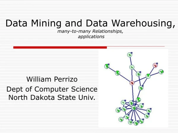
Data on a Graph: Old Hat? • Common Topics • Analyze edge structure • Google • Biological Networks • Sub-graph matching • Chemistry • Visualization • Focus on graph structure • Our work • Focus on mining node data • Graph structure provides connectivity
Protein-Protein Interactions • Protein data • From Munich Information Center for Protein Sequences (also KDD-cup 02) • Hierarchical attributes • Function • Localization • Pathways • Gene-related properties • Interactions • From experiments • Undirected graph
Questions • Prediction of a property (KDD-cup 02: AHR*) • Which properties in neighbors are relevant? • How should we integrate neighbor knowledge? • What are interesting patterns? • Which properties say more about neighboring nodes than about the node itself? But not: *AHR: Aryl Hydrocarbon Receptor Signaling Pathway
Possible Representations • OR-based • At least one neighbor has property • Example: Neighbor essential true • AND-based • All neighbors have property • Example: Neighbor essential false • Path-based (depends on maximum hops) • One record for each path • Classification: weighting? • Association Rule Mining: Record base changes AHR essential AHR essential AHR not essential
Association Rule Mining • OR-based representation • Conditions • Association rule involves AHR • Support across a link greater than within a node • Conditions on minimum confidence and support • Top 3 with respect to support: (Results by Christopher Besemann, project CSci 366)
Classification Results • Problem (especially path-based representation) • Varying amount of information per record • Many algorithms unsuitable in principle • E.g., algorithms that divide domain space • KDD-cup 02 • Very simple additive model • Based on visually identifying relationship • Number of interacting essential genes adds to probability of predicting protein as AHR
KDD-Cup 02: Honorable Mention NDSU Team
SubCell-Location Myta Ribo Nucl Ribo 17, 78 12, 60 Mi, 40 1, 48 10, 75 0 0 7, 40 0 14, 65 0 0 16, 76 0 9, 45 Pl, 43 Function apop meio mito apop StopCodonDensity .1 .1 .1 .9 PolyA-Tail 1 1 0 0 Organism Species Vert Genome Size (million bp) Gene Dimension Table g0 g1 g2 g3 o0 human Homo sapiens 1 3000 Organism Dimension Table o1 fly Drosophila melanogaster 0 185 o2 1 1 1 1 1 0 0 1 0 1 0 0 1 0 1 1 o3 0 1 0 1 1 0 0 1 0 1 0 1 1 0 0 0 yeast Saccharomyces cerevisiae 0 12.1 e0 1 0 1 1 0 1 1 1 1 1 0 1 1 0 1 0 e0 mouse Mus musculus 1 3000 e1 e1 e2 e2 e3 LAB PI UNV STR CTY STZ ED AD S H M N e3 Experiment Dimension Table (MIAME) 3 2 a c h 1 2 2 b s h 0 2 4 a c a 1 2 4 a s a 1 Gene-OrgDim Tablechromosome,length Gene-Experiment-Organism Cube 3-D gene expression cube
Protien Interaction Pyramid (2-hop interactions) SubCell-Location Myta Ribo Nucl Ribo g0 g1 g2 g3 g0 g0 1 0 0 1 g1 0 1 1 g2 0 1 0 1 g3 1 0 g1 0 1 1 0 1 0 1 0 1 g2 1 0 0 0 1 0 0 g3 Function apop meio mito apop StopCodonDensity .1 .1 .1 .9 Gene Dimension Table PolyA-Tail 1 1 0 0 Myta Ribo Nuc l apop Me i o Mi to SCD 1 SCD 2 SCD 3 SCD 4 Poly-A G E N E 1 0 0 1 0 1 0 0 0 1 1 g1 0 1 0 0 1 0 0 0 0 1 1 g2 0 0 0 1 0 0 1 0 0 0 1 0 g3 0 1 0 1 0 0 1 0 0 1 0 g4 Gene Dimension Table (Binary)
