Download
1 / 1
10 likes | 62 Views
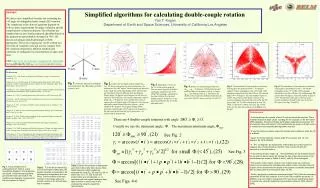
We present new formulae for evaluating 3-D earthquake double couple rotation angles, offering simpler solutions than previous methods. The equations can be easily implemented in a few lines of code, enabling comparison of earthquake solutions. Published by GJI.

E N D
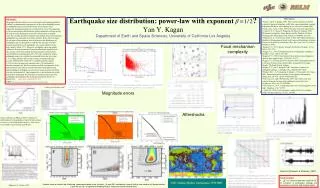
AbstractWe derive new, simplified formulae for evaluating the 3-D angle of earthquake double couple (DC) rotation. The complexity of the derived equations depends on both accuracy requirements for angle evaluation and the completeness of desired solutions. The solutions are simpler than my previously proposed algorithm based on the quaternion representation designed in 1991. We discuss advantages and disadvantages of both approaches. These new expressions can be written in a few lines of computer code and used to compare both DC solutions obtained by different methods and variations of earthquake focal mechanisms in space and time. URL: http://scec.ess.ucla.edu/~ykagan/dc3d_index.html To be published by GJI: doi: 10.1111/j.1365-246X.2007.03538.x Simplified algorithms for calculating double-couple rotationYan Y. Kagan Department of Earth and Space Sciences, University of California Los Angeles • References • Altmann, S. L., 1986. Rotations, Quaternions and Double Groups, Clarendon Press, Oxford, pp. 317. • Ekstr"om, G., A. M. Dziewonski, N. N. Maternovskaya & M. Nettles, 2005. Global seismicity of 2003: Centroid-moment-tensor solutions for 1087 earthquakes, Phys. Earth Planet. Inter., 148(2-4), 327-351. • Frohlich, C., 1992. Triangle diagrams: ternary graphs to display similarity and diversity of earthquake focal mechanisms, Phys. Earth Planet. Inter., 75, 193-198. • Hanson, A. J., 2005. Visualizing Quaternions, San Francisco, Calif., Elsevier, pp. 498. • Jost, M. L., & R. B. Herrmann, 1989. A student's guide to and review of moment tensors, Seismol. Res. Lett., 60(2), 37-57. • Kagan, Y. Y., 1991. 3-D rotation of double-couple earthquake sources, Geophys. J. Int., 106(3), 709-716. • Kagan, Y. Y., 2003. Accuracy of modern global earthquake catalogs, Phys. Earth Planet. Inter., 135(2-3), 173-209. • Kagan, Y. Y., 2005. Double-couple earthquake focal mechanism: Random rotation and display, Geophys. J. Int., 163(3), 1065-1072. • Kagan, Y. Y., and D. D. Jackson (2000), Probabilistic forecasting of earthquakes, Geophys. J. Int., 143, 438-453. • Kuipers, J. B., 2002. Quaternions and Rotation Sequences: A Primer with Applications to Orbits, Aerospace and Virtual Reality, Princeton, Princeton Univ. Press., 400 pp. • Matsumoto, T., Y. Ito, H. Matsubayashi, & S. Sekiguchi, 2006. Spatial distribution of F-net moment tensors for the 2005 West Off Fukuoka Prefecture Earthquake determined by the extended method of the NIED F-net routine, Earth Planet. Space, 58(1), 63-67. Fig. 1. Schematic diagram of earthquake focal mechanism. The right-hand coordinate system is used. Fig. 2. Isolines for maximum rotation angles ( Eq. 20, shown in degrees) for various directions of a rotation axis for a DC source. The axis angles are shown at octant equal-area projection (Kagan 2005). Dashed lines are boundaries between different focal mechanisms. Plunge angles 30 degrees and 60 degrees for all axes are shown by thin solid lines. The smallest maximum rotation angle ( = 90 degrees) is for rotation pole at any of eigenvectors, the largest angle (120 degrees) is for the pole maximally remote from all the three vectors -- in the middle of the diagram. The isogonal (Kagan 2005) maximum rotation angle (109.5 degrees) corresponds to the pole position between any two eigenvectors -- at remote ends of dashed lines. Fig. 3. Dependence of error in Eq. 25 on the rotation angle . Dots are errors for pairs of shallow earthquake solutions in the 1977-2004 CMT catalogue, separated by less than 100 km, N is the total number of pairs. Solid curve is the theoretical estimate (Eq. 27) of the maximum error. Fig. 4. Isolines for rotation angles difference ( , in degrees). Octant projection and auxiliary lines are the same as in Fig. 2. Angles ( ) are displayed in Fig. 2. The angles are shown in the system of coordinates formed by the axes of the first DC source (see Eqs. 34 and 35). Fig. 5. The distribution of rotation poles in solutions with negative dot products for M >= 5.0 shallow (depth 0-70 km) earthquakes in the 1977-2004 CMT catalogue, separated by less than 100 km. The rotation angle is 90 degrees. The total number of pairs is 16,253. The position of the poles is shown in the system coordinates formed by the axes of the first DC source (Eqs. 34, 35). The rotation pole for row 2 in Table 3 is shown by a white circle (see Eq. 36 and below it). We show the positions of the tpb-axes in the plot. Fig. 6. The distribution of rotation poles in solutions with negative dot products for M >= 5.0 shallow earthquakes in the 1977-2004 CMT catalogue, separated by less than 100 km. The rotation angle is greater than 105 degrees. The total number of pairs is 2,335. The position of the poles is shown in the system coordinates formed by the axes of the first DC source (see Eqs. 34 and 35). • Conclusions • In the beginning, the equality of two DC sources should be checked. This is needed because of angle values rounding off. For example, in the 1977-2004 CMT catalogue, 35 pairs of shallow earthquakes separated by less than 100 km have the same mechanism. If the mechanisms are equal, no further action is needed and more sophisticated algorithms may fail. • If only the minimum rotation angle is needed and is relatively small, Eq. 25 is sufficient. • Again, if only the minimum rotation angle is needed, and < 90 degrees, Eq. 28 is sufficient. • If 90 degrees, the handedness of the solutions and the number of negative dot products should be checked. Then use Eq. 29 with the instructions in the text below it. • If we need all the four angles , the handedness of both solutions should be corrected to be the same. We change the sign of two dot products in four combinations (as shown in Tables 2 and 3), and Eq. 29 is used again. • The position of the rotation vectors or the rotation poles on a reference sphere can be obtained by calculating the rotation matrix. If needed, the pole position can be transformed for display in the system coordinates associated with an earthquake focal mechanism (Eqs. 34-36). • Finally, applying the quaternion technique (Kagan 1991) yields the necessary parameters for the four rotations, if one or two of the rotations are binary. In addition, as a rule, rotation sequences of DC sources are significantly easier to construct by using the quaternion representation (Kuipers 2002; Hanson 2005). There are 4 double-couple rotations with angle The maximum minimum angle, Usually we use the minimum angle, See Fig. 2 See Fig. 3 Table 3. E# are the numbers of earthquake pairs from Table 2 (the first column). Bold-faced minimum rotation angles are evaluated by using (Eq. 28) and (Eq. 29). In these rows (1, 6, 11, and 16) the dot product signs are not adjusted, i.e., is calculated with the original catalogue data. Italic numbers in rows 9 and 10 are evaluated by using the quaternion representation. Fig. 7. Focal mechanisms of earthquakes from Table 2. Lower hemisphere diagrams of focal spheres are shown, compressional quadrants (around the t-axis) are shaded. The numbers near diagrams correspond to the row numbers in Table 2. Table 2. is the third invariant (Eq. 7) of an orientation DCM matrix; the positive invariant corresponds to the right-handed configuration and vice versa. The first number in the axis columns is the plunge alpha, the second number is the azimuth beta, both in degrees. See Figs. 4-6