Back Propagation through time

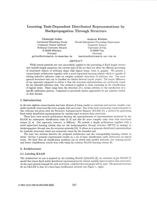
1. Learning Task-Dependent Distributed Representations by Backpropagation Through Structure Christoph Goller Automated Reasoning Group Computer Science Institute Technical University Munich D-80290 Miinchen Germany ,goller@informatik.tu-muenchen.de Andreas Kuchler Neural Information Processing Department Computer Science University of Ulm D-89069 Ulm Germany kuechler0informatik.uni-ulm.de ABSTRACT While neural networks are very successfully applied to the processing of fixed-length vectors and variable-length sequences, the current state of the art does not allow the efficient processing of structured objects of arbitrary shape (like logical terms, trees or graphs). We present a connectionist architecture together with a novel supervised learning scheme which is capable of solving inductive inference tasks on complex symbolic structures of arbitrary size. The most general structures that can be handled are labeled directed acyclic graphs. The major difference of our approach compared to others is that the structure-representations are exclusively tuned for the intended inference task. Our method is applied to tasks consisting in the classification of logical terms. These range from the detection of a certain subterm to the satisfaction of a specific unification pattern. Compared to previously known approaches we got superior results on that domain. 1. Introdluction In the late eighties connectionism had been blamed of being unable to represent and process complex com- posite symbolic structures like trees, graphs, lists and terms. One of the most convincing counterexamples to this criticism was given with the Recursive Autoassociative Memory (RAAM) [7], a method for generating fixed-width distributed representations for variable-sized recursive data structures. There have been several publications showing the appropriateness of representations produced by the RAAM for subsequent classification tasks [3, 61 and also for more complex tasks even with structured output 12, 41. Our approach, however, is different. We present a simple architecture together with a novel supervised learning scheme that we call backpropagation through structure (BPTS) in analogy to backpropagation through t i m e for recurrent networks [lo]. It allows us to generate distributed representations for symbolic structures which are exclusively tuned for the intended task. The next two sections describe the proposed architecture and the corresponding learning scheme in detail. Section 4 presents experimental results on a set of basic classification tasks (detectors) on logical terms. We show that all classification problems can be solved with smaller networks, less training epochs and better classification results than with using the ordinary RAAM learning scheme [6]. 2. Architecture 2.1. Labeling RAAM The architecture we use is inspired by the Labeling RAAM (LRAAM) [SI, an extension of $he RAAM [7] model that learns fixed-width distributed representations for labeled variable-sized recursive data structures. As the most general example for such structures, a labeled directed graph will be used. The general structure for an LRAAM is that of a three-layer feedforward network (see Figure I, right). 347 0-7803-32 10496 $4.0001 996 IEEE

2. (n+km) uniLc hranch 2 (nckni) unib hranch 2 hranch k lahel hranch 1 hranch k hranch I Iakl I m units 1 m units n units Encoder m units Hidden Hidden 0 0 Decoder 0 I m units I m units n units output Fig. 1: The Folding Architecture (left side) and the standard LRAAM (right side). The idea is to obtain a compressed representation (hidden layer activation) for a node of a labmd directed graph by allocating a part of the input (output) of the network to represent the label and the rest to represent its subgraphs with a fixed maximum number of subgraphs IC using a special representation for the empty subgraph. The network is trained by backpropagation in an autoassociative way using the compressed representations recursively. As the representations are consistently updated during the training, the training set is dynamic (moving target), starting with randomly chosen representations. 2.2. Folding Architecture For reasons of clarity and simplicity we will concentrate on inference tasks consisting of the classification of logical terms in the following. However note, that our architecture together with the corresponding training procedure (Section 3) could be easily extended to handle inference tasks of more complex nature. Figure 1 (left side) shows the folding architecture we use. The first two layers occupy the role of the standard LRAAM encoder part, the hidden units are connected to a simple sigmoid feedforward layer, in our case just one unit for classification. For the classification of a new structure, the network is virtually unfolded (just as in Figure 3) to compute the structure’s representation, which is then used as input for the classifier. This would be done in the same way for LRAAM-derived representations. However, we use the virtual unfolding of the network also for the learning phase and propagate the classification error through the whole virtually unfolded network, instead of using a decoder part for finding unique representations. The idea behind this is, that for many inference tasks unique representations are not necessary as long as the information needed for the inference task is represented properly. Our learning scheme is completely supervised without moving targets. 3. Backpropagation Through Structure The principle idea of using recursive backpropagation-like learning procedures for symbolic tree-processing has been mentioned first in [l, 91. We assume in the following the reader to be familiar with the standard backpropagation algorithm (BP) and its variant backpropagation through time (BPTT) [lo] that is used to train recurrent network models. For the sake of brevity we will only be able to give a sketch of the underlying principles of our approach. Refer to 151 for a detailed discussion and formal specification of the given algorithms. Let us first have a closer look on the representation of structures we want to process. All kinds of recursive symbolic data structures we aim at can be mapped onto labeled directed acyclic graphs (DAGS). For example choosing a DAG-representation for a set of logical terms (see Figure 2)- that allows to represent different occurrences of a (sub-)structure only as one node - may lead to a considerable (even exponential) reduction of space complexity. But this complexity reduction also holds for the time complexity of training. For the LRAAM training as well as for BPTS (as we will show in the following two sections) the number of forward and backward phases per epoch is linear to the number of nodes in the DAG-representation of the training set. 348

3. Terms Tree-Representation Dag-Representation Fig. 2: Tree and DAG representation of a set of terms. 3.1. BPTS for flrees For reasons of simplicity we first restrict our considerations to tree-like structures. In the fomoard phase the encoder (Figure 1, left) is used to compute a representation for a given tree in the same way as in the plain LRAAM. The following metaphor helps us to explain the backward phase. Imagine the encoder of the folding architecture is virtually unfolded (with copied weights) according to the tree structure (see Figure 3). Now the error passed from the classifier to the hidden layer is propagated through the unfolded encoder network. Fig. 3: The Encoder unfolded by the structure f(X, g(a, Y)). With a similar argument as for BPTT (lo] we can see, that the exact gradient is computed. The exact formulation is given below: For each (sub-)tree t, t.z E Rn+km is the input vector of the encoder, & E R " the vector of (error-) deltas for t's representation, and (t.z, t') the projection of t.z onto t's subtree t'. Let further W be the encoder matrix, f ' the derivative of the transfer function and 0 the multiplication of two vectors by components. AW is calculated as sum over all (sub-)trees (1). The 6 ; the & of the one definite parent node t oft' back according to (2): AW = ~ C g ( t . z ) ~ (1) t for each subtree t' is calculated by propagating (W'& 0 f'(t.z), t') = (2) 6 1 For each (sub-)tree in the training set one epoch requires exactly one forward and one backward phase through the encoder. The training set is static (no moving target). 3.2. BPTS for DAGS However, if we use a DAG-representation and represent a (sub-)structure t only as one node independently from the number of its occurrences, then there may be different & in (1) and (2) for each occurrence of t. We call this situation a delta conflict. Suppose the (sub-)structures ti and tj are identical. Of course this means that corresponding substruc- tures within ti and t j are identical too. This clearly gives us ti.x = tj.z, but we may have St, # St, e - . . 349

4. problem name lbloccl long termoccl symbols used #subterms (tr.,test) depth (pos.,neg.) rules for #terms (tr.,test) positive examples. f/2 i/l a/O b/O c/o no occurrence of label c (259,141) (444,301) (5,5) f/2 i/l a/O b/O C/O the (sub)terms i(a) or f(b,c) occur somewhere the (sub)terms i(a) or f(b,c) occur somewhere instances of f(X,f(a,Y)) instances of f(X,f(a,Y)) (173,70) (179,79) (22) I termoccl very long inst4 inst4 long inst5 simil neg. f/2 i/l a/O b/O c/o (280,120) (559,291) (6,6) f/2 a/O b/O c/o f/2 a/O b/O c/o (175,80) (290,110) (179,97) (499,245) (3J) ( 7 N instances of t(a,i(X),f(b,Y)), g(i(f(b,X)),j(Y)) or g(i(X),i(f(b,Y))) instances of f(j(X),f(a,Y)), g(f(a,Y),i(X)) or t/3 f/2 g/2 i/l j/l a/0 b/O C/O d/O (259,141) (1394,776) (7,7) instoccl t/3 f/2 g/2 i/l j / l a/O b/O C/O d/O (1247,497) (7,6) (217,83) i(j(f(a,Y))) occur somewhere instances of f(X,X) instances of f(X,)o f/2 a/O b/O C/O f/2 a/0 b/O c/o instl instl long inst7 (235,118) (403,204) (3,2) (6,6) (200,83) (202,98) t/3 f/2 g/2 i/l j/l a/O b/O c/o d/O instances of t(i(X),g(X,b),b) (191,109) (1001,555) (6,6) Table: 1: Description of the set of classification problems involving logical terms For calculating AW we only need the sum of 6 ; ‘ and 6 ; . This is shown by the following transformation of (1) which holds because of the linearity of matrix multiplication: The &I’S of corresponding children t’ oft, and t, can be calculated more efficiently too, by propagating the sum of 6yx and 6 ; back in (2). A similar transformation (linearity of n, (2) shows this. Summing up all different 6’s coming from each occurrence of a (sub-)structure is a correct (steepest gradient) solution of the delta conflict and enables a very efficient implementation of BPTS for DAGS. We just have to organize the nodes of the training set in a topological order. The forward phase starts with the leaf-nodes and proceeds according to the reverse ordering - ensuring that representations for identical substructures have to be computed only once. The backward phase follows the topological order beginning at the root-nodes. In this way the 6’s of all occurrences of a node are summed up before that node is processed. Again for each node in the training set one epoch requires exactly one forward and one backward phase through the encoder. Similar to standard BP, BPTS can be used in batch or in online mode. BPTS- batch updates the weights after the whole training set has been presented. By the optimization techniques discussed above (&summation and DAG-representation) each node has to be processed only once per epoch. This does not hold for online mode because the weights are updated immediately after one structure has been presented and therefore substructures have to be processed for each occurrence separately. @ and matrix multiplication) for 4 . Experiments The characteristics of each term classification problem we used to evaluate our approach are summarized in Table 1. The set of problems is an extension of the one used in [6]. They range from the detection of a certain subterm to the satisfaction of a specific unification pattern. The second column reports the set of symbols (with associated arity) compounding the terms, the third column shows the rule(s) used to generate the positive examples with upper case letters representing all-quantified logical variables. The fourth column reports the number of terms in the training and test set respectively, the fifth column the number of subterms (using the DAG-representation as described in Section 3), and the last column the 350

5. [long c % T r . % Ts. % Dec.-Enc. Problem Method Topology #L Learning Par. 7 I #epochs #H C P A lraamc 0 batch ~online A 0 lbloccl instl c c [long 8 8 8 8 8 8 6 6 6 6 6 6 6 6 6 6 6 6 13 13 13 8 8 35 2 2 25 5 5 35 3 5 45 3 3 35 3 3 35 3 3 40 3 3 6 6 3 5 6 7 0.2 0.001 0.001 0.1 0.001 0.001 0.2 0.001 0.005 0.2 0.005 0.005 0.2 0.001 0.001 0.2 0.003 0.005 0.1 0.01 0.01 0.001 0.001 0.001 0.001 0.001 0.001 0.001 0.5 - 0.6 0.6 0.2 0.6 0.6 0.5 0.6 0.6 0.5 0.6 0.6 - 0.5 0.6 0.6 0.5 0.6 0.6 0.2 0.6 0.6 0.6 0.6 0.6 0.6 0.6 0.6 - - 4.25 100 99.61 100 98.84 97.69 100 97 97 97.5 94.55 95.56 98.52 100 100 100 100 100 100 100 100 100 99.64 99.29 94.21 98.06 96.31 97.24 98.58 100 100 94.29 95.71 94.29 93.98 93.98 91.57 90.82 92.86 94.90 100 100 100 100 100 100 100 100 100 98.33 94.17 93.62 92.20 80.72 72.29 11951 108 444 27796 5271 6925 10452 278 213 80000 4250 465 1759 37 68 6993 150 27 6158 10 57 3522 2263 1558 198 338 369 termoccl 0.1 100 - A 0 0.06 100 - inst 1 A 0 0.005 36.14 A 0 B A 0 m A 0 instl 0.005 98.86 - - 0.005 8.97 c c inst7 0.01 1.05 - - termoccl very long inst5 simil neg. iinstoccl c 0 8 I 13 13 13 13 U 0 Table: 2: The best results obtained for each classification problem. maximum depth' of terms. For each problem about the same number of positive and negative examples is given. 130th positive and negative examples have been generated randomly. Training and test sets are disjoint and have been generated by the same algorithm. Table 2 shows the best results we have obtained. The different columns describe the problem class, the method used, the topology of the network ( + #L, number units in the labels, the representations), training parameters ( a 7, learning parameter, +- p, momentum), the performance ( * %Tr./%Ts. the percentage of terms of the training/test set correctly classified) and the number of learning epochs needed to achieve these results. We have applied and compared BPTS in online (+ U) and batch (=s- 0) mode on each problem instance. For online mode, the training set was presented in the same order every epoch. Only one learning parameter 7, one momentum p = 0.6 and one transfer function tanh was used throughout the whole three-layered network architecture. Since 'we have considered two-class decision problems the output unit was taught with values -1.0/1.0 for negative/positive membership. The classification performance measure was computed by fixing the decision boundary at 0. The performance of the folding architecture with BPTS is listed together with the results of a combined LRAAM-classifier2 (LRAAMC) architecture (* A) whenever results for the LRAAMC were available [6]. A more detailed discussion of the problem classes viewed in relation to the results can be found in [5]. Our folding architecture supplied with BPTS leads to nearly the same or slightly better classification performance than the LRAAMC approach. But this has been achieved by a topology which uses one #H, number of units for 'We define the depth of a term as the maximum number of edges between the root and leaf nodes in the term's LDAG- representation. 2LRAAMC uses a special dynamic pattern selection strategy for network training and applies different learning parameters to the LRAAM (a 7) and the classifier (3 e). 35 1

6. order of magnitude less hidden units and by a learning procedure which needs more than one order of magnitude less training epochs to converge to the same performance. Beside complexity considerations (see section 3.2) BPTS-batch seems to have no significant advantages over BPTS-online at the current stage of our investigations based on the given experimental results. Why is the folding architecture together with BPTS superior to the LRAAMC? Obviously, the LRAAMC has to solve the additional task of developing unique representations, i.e. to minimize the encoding-decoding error ( j % Dec.-Enc., in Table 2). This may be much more difficult and sometimes contradictory to the classification task. Furthermore, as the error from the classifier is not propagated recursively through the structure in the LRAAMC, the exact gradient is not computed and (in contrast to our approach) the representations of subterms are not optimized directly for the classification task concerning their parents. 5. Conclusion By using the folding architecture together with BPTS the encoding of structures is melted with further inference into one single process. We have shown that our method is really superior over previously known approaches, at least on the set of term-classification problems presented here. In order learn more about the generalization capabilities of the architecture it will be important to analyze the generated representations. We plan to experiment with more complex architectures (e.g. additional layers in the encoder or in the classifier) and with examples coming from “real” applications. One we are currently working on is a hybrid (symbolic/connectionist) reasoning system, in which our methods will be used to learn search control heuristics from examples. Acknowledgment This research was supported by the German Research Foundation (DFG) under grant No. Pa 268/10-1. Our thanks to Alessandro Sperduti for helpful comments and to Andreas Stolcke for providing us with his RAAM implementation. References [l] G. Berg, “Connectionist Parser with Recursive Sentence Structure and Lexical Disambiguation,” in Proceedings of the AAAI 92, pp. 32-37, 1992. [2] D. S. Blank, L. A. Meeden, and J. B. Marshall, “Exploring the Symbolic/Subsymbolic Continuum: A Case Study of RAAM,” in The Symbolic and Connectionist Paradigms: Closing the Gap, (J. Dinsmore, ed.), LEA Publishers, 1992. [3] V. Cadoret, “Encoding Syntactical Trees with Labelling Recursive Auto-Associative Memory,” in Proceedings of the ECAI 94, pp. 555-559, 1994. [4] L. Chrisman, “Learning Recursive Distributed Representations for Holistic Computation,” Connection Science, no. 3, pp. 345-366, 1991. [5] C. Goller and A. Kuchler, “Learning Task-Dependent Distributed Representations by Backpropagation Through Structure,” AR-report AR-95-02, Institut fur Informatik, Technische Universitat Munchen, 1995. [6] C. Goller, A. Sperduti, and A. Starita, “Learning Distributed Representations for the Classification of Terms,” in Proceedings of the IJCAI 95, pp. 509-515, 1995. [7] J. B. Pollack, “Recursive Distributed Representations,” Artificial Intelligence, vol. 46, no. 1-2, 1990. [8] A. Sperduti, “Encoding of Labeled Graphs by Labeling RAAM,” in NIPS 6, (J. D. Cowan, G. Tesauro, and J. Alspector, eds.), pp. 1125-1132, 1994. [9] A. Stolcke and D. Wu, “Tree Matching with Recursive Distributed Representations,” Tech. Rep. TR- 92-025, International Computer Science Institute, Berkeley, California, 1992. [lo] P. J. Werbos, “Backpropagation Trough Time: What it Does and How to Do it,” Proceedings of the IEEE, vol. 78, pp. 1550-1560, Oct. 1990. 352