Download
1 / 60
600 likes | 1.36k Views
Digital Signal Processing for Communications and Information Systems (DSP-CIS). Marc Moonen Dept. E.E./ESAT, K.U.Leuven marc.moonen@esat.kuleuven.be www.esat.kuleuven.be / scd /. Chapter-1 : Introduction. Part-1: Aims/Scope Why study DSP ?

E N D
Digital Signal Processingfor Communications and Information Systems(DSP-CIS) Marc Moonen Dept. E.E./ESAT, K.U.Leuven marc.moonen@esat.kuleuven.be www.esat.kuleuven.be/scd/
Chapter-1 : Introduction • Part-1: • Aims/Scope Why study DSP ? DSP in applications : GSM example • Overview • Activities Lectures: Course Notes/Literature Exercise Sessions: Acoustic Modem Project Exam • Part-2: • Acoustic Modem Project
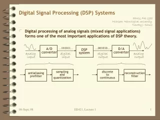
Why study DSP ? • Analog Systems vs. Digital Systems - Can translate (any) analog (e.g. filter) design into digital - Going `digital’ allows to expand functionality/flexibility/… (e.g. how would you do analog speech recognition ? analog audio compression ? …? ) OUT OUT IN 2 IN +2 A/D D/A =4
Why study DSP ? • Start with one `DSP in applications’ example: • DSP in mobile communications (GSM) • Main message: Consumer electronics products (and many other systems) have become ‘supercomputers’(Mops/sec…Gops/sec), packed with mathematics & DSP functionalities…
DSP in applications : GSM Cellular mobile telephony (e.g. GSM) • Basic network architecture : -Country covered by a grid of cells -Each cell has a base station -Base station connected to land telephone network and communicates with mobiles via a radio interface -Digital communication format
DSP in applications : GSM • DSP for digital communications (`physical layer’ ) : • A common misunderstanding is that digital communications is `simple’…. • While in practice… .99,.01,.96,.95,.07,… Transmitter 1,0,1,1,0,… Channel Receiver x + x decision 1,0,1,1,0,… 1/a a noise
Transmitter 1,0,1,1,0,… Receiver `Multipath’ Channel ?? + noise DSP in applications : GSM • DSP for digital communications (`physical layer’ ) : • While in practice… • This calls for channel modeling + compensation (equalization) !! .59,.41,.76,.05,.37,… 1,0,1,1,0,…
Δ Δ Δ Δ Δ Δ Δ Δ Δ Δ a `Multipath’ Channel b c ≈ + + d e DSP in applications : GSM • GSM Channel Estimation/Compensation • Multi-path channel is modeled with short (3…5 taps) FIR filter H(z)= a+b.zˉ¹+c.z ˉ²+d.z ˉ³+e.z ˉ(interpretation?) 4
Δ Δ Δ Δ Δ Δ Δ Δ Δ Δ a b c + d e DSP in applications : GSM • GSM Channel Estimation/Compensation (continued) • Multi-path channel is modeled with short (3…5 taps) FIR filter H(z)= a+b.zˉ¹+c.z ˉ²+d.z ˉ³+e.z ˉ 4 OUT[k] IN[k] =convolution
DSP in applications : GSM • GSM Channel Estimation/Compensation (continued) • Channel coefficients (a,b,c,d,e) are identified in receiver based on transmission of pre-defined training sequences (TS), in between data bits. Problem to be solved at receiver is: `given channel input (=TS) and channel output (=observed), compute channel coefficients’ This leads to a least-squares parameter estimation See PART-III on ‘Optimal Filtering’ Carl Friedrich Gauss (1777 – 1855)
DSP in applications : GSM • GSM Channel Estimation/Compensation (continued) • Channel coefficients (cfr. a,b,c,d,e) are identified in receiver based on transmission of pre-defined training sequences (TS), in between data bits. • Channel model is then used to design suitable equalizer (`channel inversion’), or (better) to reconstruct transmitted data bits based on maximum-likelihood sequence estimation (e.g. `Viterbi decoding’). • Channel is highly time-varying (e.g. terminal speed 120 km/hr !) => All this is done at `burst-rate’ (+- 100 times per sec). = SPECTACULAR !!
DSP in applications : GSM • GSM Channel Estimation/Compensation • GSM Speech Coding • Original `PCM-signal has 64kbits/sec =8 ksamples/sec*8bits/sample • Aim is to reduce this to <11kbits/sec, while preserving quality! • Coding based on speech generation model (vocal tract,…), where model coefficient are identified for each new speech segment (e.g. 20 msec). • This leads to a least-squares parameter estimation (again), executed +- 50 times per second. Fast algorithm is used, e.g. `Levinson-Durbin’ algorithm. See PART-III on ‘Optimal Filtering’. • Then transmit model coefficients instead of signal samples. • Synthesize speech segment at receiver (should `sounds like’ original speech segment). = SPECTACULAR !!
DSP in applications : GSM • GSM Channel Estimation/Compensation • GSM Speech Coding • GSM Multiple Access Schemes • Capacity increase by time & frequency `multiplexing’ • FDMA : e.g. 125 frequency channels for GSM/900MHz • TDMA : 8 time slots(=users) per channel, `burst mode’ communication (PS: in practice, capacity per cell << 8*125 ! ) See PART-II on ‘Filter Banks & Transmultiplexers’ • Etc.. = BOX FULL OF DSP/MATHEMATICS !! (for only €25)
DSP in applications : Other… • Digital Communications Wireline (xDSL,Powerline), Wireless (GSM, 3G, Wi-Fi, WiMax CDMA, MIMO-transmission,..) • Speech Speech coding (GSM, DECT, ..), Speech synthesis (text-to-speech), Speech recognition • Audio Signal Processing Audio Coding (MP3, AAC, ..), Audio synthesis Editing, Automatic transcription, Dolby/Surround, 3D-audio,. • Image/Video • …
DSP in applications Enabling Technology is • Signal Processing 1G-SP: analog filters 2G-SP: digital filters, FFT’s, etc. 3G-SP: full of mathematics, linear algebra, statistics, etc... • Micro-/Nano-electronics • ... Signals&Systems course (JVDW) DSP-I (PW) DSP-CIS
DSP-II Aims/Scope • Basic signal processing theory/principles filter design, filter banks, optimal filters & adaptive filters …as well as… • Recent/advanced topics robust filter realization, perfect reconstruction filter banks, fast adaptive algorithms, ... • Often `bird’s-eye view’ skip many mathematical details (if possible… ) selection of topics (non-exhaustive)
Overview (I) • INTRO : Chapter-1 Chapter-2: Signals and Systems Review • Part I : Filter Design & Implementation Chapter-3: IIR & FIR Filter Design Chapter-4: Filter Realization Chapter-5: Filter Implementation
Overview (II) • Part II: Filter Banks & Subband Systems Chapter-6: Filter Banks Intro/Applications (audio coding/CDMA/…) Chapter-7: Filter Banks Theory Chapter-8: DFT-modulated Filter Banks Chapter-9: Special Topics (frequency-domain processing, wavelets…) 3 subband processing 3 G1(z) H1(z) OUT IN 3 subband processing 3 G2(z) H2(z) + 3 subband processing 3 G3(z) H3(z) 3 subband processing 3 G4(z) H4(z)
Overview (III) • Part III : Optimal & Adaptive Filtering Chapter-10: Optimal/Wiener Filters Chapter-11: Adaptive Filters/Recursive Least Squares Chapter-12: Adaptive Filters/LMS Chapter-13: `Fast’ Adaptive Filters Chapter-14: Kalman Filters
Activities : Lectures Lectures: 14 * 2 hrs PS: Time budget = (14*2hrs)*4 = 112 hrs Course Material: • Part I-II-III:Slides (use version 2011-2012 !!) ...download from DSP-CIS webpage • Part III: `Introduction to Adaptive Signal Processing‘ (Marc Moonen & Ian.K. Proudler) = support material, not mandatory ! …(if needed) download from DSP-CIS webpage
Literature / Campus Library Arenberg • A. Oppenheim & R. Schafer `Digital Signal Processing’(Prentice Hall 1977) • L. Jackson `Digital Filters and Signal Processing’(Kluwer 1986) • P.P. Vaidyanathan `Multirate Systems and Filter Banks’(Prentice Hall 1993) • Simon Haykin `Adaptive Filter Theory’(Prentice Hall 1996) • M. Bellanger `Digital Processing of Signals’(Kluwer 1986) • etc... Part-I Part-II Part-III
Literature / DSP-CIS Library • Collection of books is available to support course material • List/reservation via DSP-CIS webpage • Contact: beier.li@esat
Activities : Exercise Sessions `Acoustic Modem Project’ • Digital communication over an acoustic channel (from loudspeaker to microphone) • FFT/IFFT-based modulation format : OFDM (as in ADSL/VDSL, WiFi, …) • Channel estimation, equalization, etc… Rx Tx A-to-D D-to-A +filtering +amplif. +filtering +… ..more on this in Part-2
Activities : Exercise Sessions `Acoustic Modem Project’ • Runs over 8 weeks • Each week • 1 PC/Matlab session (supervised, 2.5hrs) • 2 ‘Homework’ sesions (unsupervised, 2*2.5hrs) PS: Time budget = 8*(2.5hrs+5hrs) = 60 hrs • ‘Deliverables’ after week 2, 4, 6, 8 • Grading: based on deliverables, evaluated during sessions • TAs:alexander.bertrand@esat(English+Dutch) beier.li@esat(English+Chinese) paschalis.tsiaflakis@esat(English+Greek+Dutch) pepe.gilcacho@esat(English+Spanish) PS: groups of 2
Activities : Exam • Oral exam, with preparation time • Open book • Grading : 5 pts for question-1 5 pts for question-2 5 pts for question-3 ps: 1 question (could be) referring to Acoustic Modem Project 5 pts for Acoustic Modem Project evaluation ___ = 20 pts
homes.esat.kuleuven.be/~pepe/dsp-cis/2011-2012 • Contact: pepe.gilcacho@esat • Slides • Project info/schedule • Exams • DSP-CIS Library • FAQs (send questions to pepe.gilcacho@esat or marc.moonen@esat )
Chapter-1 : Introduction • Part-1: • Aims/Scope Why study DSP ? DSP in applications : GSM example • Overview • Activities Lectures: Course Notes/Literature Exercise Sessions: Acoustic Modem Project Exam • Part-2: • Acoustic Modem Project
Discrete-time receiver signal (sampling rate Fs, e.g. 10kHz) Discrete-time transmit signal (sampling rate Fs, e.g. 10kHz) Rx Tx A-to-D D-to-A +filtering +amplif. +filtering +… Introduction / Acoustic Modem • Will consider digital communications over acoustic channel:
Introduction / Acoustic Modem • Will consider digital communications over acoustic channel: Discrete-time receiver signal (sampling rate Fs, e.g. 10kHz) Discrete-time transmit signal (sampling rate Fs, e.g. 10kHz) Rx Tx A-to-D D-to-A +filtering +amplif. +filtering +… This will be the easy part…
Introduction / Acoustic Modem • Will consider digital communications over acoustic channel: …straightforwardly realized (in Matlab/Simulink with `Real-Time Workshop’, see below) Discrete-time receiver signal (sampling rate Fs, e.g. 10kHz) Discrete-time transmit signal (sampling rate Fs, e.g. 10kHz) Rx Tx A-to-D D-to-A +filtering +amplif. +filtering +… means we do not have to deal with hardware issues, RF components, etc.
Introduction / Acoustic Modem • Will consider digital communications over acoustic channel: …and will be modeled by a linear discrete-time transfer function (see below) Discrete-time receiver signal (sampling rate Fs, e.g. 10kHz) Discrete-time transmit signal (sampling rate Fs, e.g. 10kHz) H(z) Rx Tx A-to-D D-to-A +filtering +amplif. +filtering +…
Introduction / Acoustic Modem • Will consider digital communications over acoustic channel: Discrete-time receiver signal (sampling rate Fs, e.g. 10kHz) Discrete-time transmit signal (sampling rate Fs, e.g. 10kHz) Rx Tx A-to-D D-to-A +filtering +amplif. +filtering +… This is the interesting part… (where we will spend most of the time)
Introduction / Acoustic Modem • Will use OFDM as a modulation format • OFDM/DMT is used in ADSL/VDSL, WiFi, DAB, DVB … • OFDM heavily relies on DSP functionalities (FFT/IFFT, …) Orthogonal frequency-division multiplexing From Wikipedia, the free encyclopedia Orthogonal frequency-division multiplexing (OFDM), essentially identical to (…) discrete multi-tone modulation (DMT), is a frequency-division multiplexing (FDM) scheme used as a digital multi-carrier modulation method. A large number of closely-spaced orthogonal sub-carriers are used to carry data. The data is divided into several parallel data streams or channels, one for each sub-carrier. Each sub-carrier is modulated with a conventional modulation scheme (such as quadrature amplitude modulation or phase-shift keying) at a low symbol rate, maintaining total data rates similar to conventional single-carrier modulation schemes in the same bandwidth. OFDM has developed into a popular scheme for wideband digital communication, whether wireless or over copper wires, used in applications such as digital television and audio broadcasting, wireless networking and broadband internet access.
Rx Tx A-to-D D-to-A Introduction / Acoustic Modem Target: Design efficient OFDM based modem (Tx/Rx) for transmission over acoustic channel Specifications: Data rate (e.g. 1kbits/sec), bit error rate (e.g. 0.5%), channel tracking speed, synchronisation, …
Work Plan 8 Weeks: • Week 1: Introduction Matlab/Simulink • Week 2: Acoustic channel measurement & modeling *deliverable* • Week 3-4: OFDM transmitter/receiver design *deliverable* • Week 5-6: OFDM over acoustic channel *deliverable* • Week 7-8: OFDM with adaptive equalization *deliverable*
Week 1 / Matlab & Simulink Introduction Matlab/Simulink
Week 1 / Matlab & Simulink Will also provide basic Simulink scheme… (`Real-Time Workshop’)
Discrete-time receiver signal (sampling rate Fs, e.g. 10kHz) Discrete-time transmit signal (sampling rate Fs, e.g. 10kHz) Rx Tx A-to-D D-to-A +filtering +amplif. +filtering +… Week 2 / Channel Modeling & Evaluation Transmission channel consist of • Tx `front end’: filtering/amplification/Digital-to-Analog conv. • Loudspeaker (ps: cheap loudspeakers mostly have a non-linear characteristic ) • Acoustic channel • Microphone • Rx `front end’: filtering/Analog-to-Digital conv.
Week 2/ Channel Modeling & Evaluation Acoustic channel (`room acoustics’): Acoustic path between loudspeaker and microphone is represented by theacoustic impulse response(which can be recorded/measured) • Observe that : • first there is a dead time • then come the direct path impulse • and some early reflections, which • depend on the geometry of the room • finally there is an exponentially decaying tail called reverberation, corresponding to multiple reflections on walls, objects,...
Week 2 / Channel Modeling & Evaluation Complete transmission channel will be modeled by a discrete-time (FIR `finite impulse response’) transfer function • Pragmatic & good-enough approximation • Model order L depends on sampling rate (e.g. L=100…1000…) H(z) Rx Tx A-to-D D-to-A +filtering +amplif. +filtering +…
Week 2 / Channel Modeling & Evaluation When a discrete-time (Tx) signal x_k is sent over a channel… ..then channel output signal (=Rx input signal) y_k is =`convolution’
Week 2 / Channel Modeling & Evaluation Can now run parameter estimation experiment: • Transmit `well-chosen’ signal x_k • Record corresponding signal y_k y_k H(z) x_k Rx Tx A-to-D D-to-A +filtering +amplif. +filtering +…
Week 2 / Channel Modeling & Evaluation 3. Least squares estimation (i.e. one line of Matlab code ) Carl Friedrich Gauss (1777 – 1855)
Week 2 / Channel Modeling & Evaluation Estimated transmission channel can then be analysed… • Frequency response • Information theoretic capacity ps: noise spectrum? Claude Shannon 1916-2001
Week 3-4 / OFDM modulation DMT – Discrete Multitone Modulation OFDM – Orthogonal Frequency Division Multiplexing Basic idea is to (QAM-)modulate (many) different carriers with low-rate bit streams. The modulated carriers are summed and then transmitted. A high-rate bit stream is thus carried by dividing it into hundreds of low-rate streams. Modulation/demodulation is performed by FFT/IFFT (see below) Now 10 pages of (simple) maths/theory…
Week 3-4 / OFDM modulation 1/10 Consider modulation of a segment of a complex exponential carrier (frequency w) by a `symbol’ X_w, generating a segment of a (time-domain) signal x_k : PS: remember that modulation of sines and cosines is similar/related to modulation of complex exponentials
Week 3-4 / OFDM modulation 2/10 Modulation of N such carriers at once (with well-chosen frequencies, i.e. such that segment always has integer number of periods) is realized by means of N-point (so-called) `Inverse Discrete Fourier Transform’ (IDFT)
Week 3-4 / OFDM modulation 3/10 • PS:Note that modulates a DC signal • PS: To ensure time-domain signal is real-valued, have to choose • PS: The IDFT matrix is a cool matrix: • For any dimension N, an IDFT matrix can be constructed as given on the previous slide. • Its inverse is the so-called DFT matrix (symbol `F’). DFT and IDFT matrices are unitary (up to a scalar), i.e. • The structure of the IDFT matrix allows for a cheap (complexity N.logN instead of N.N) algorithm to compute the matrix-vector product on the previous slide (IFFT `inverse fast Fourier transform’).
Week 3-4 / OFDM modulation 4/10 • So this will be the basic modulation operation at the Tx : • The X_w’s will be (QAM-symbols) defined by the input bit stream • The time-domain signal segments are transmitted over the channel, one after the other. At the receiver, demodulation will be done with an inverse operation (see below: vector of received samples is multiplied by F, based on FFT `fast Fourier transform ). Imag(Xi) Real(Xi)
Week 3-4 / OFDM modulation 5/10 • Sounds simple, but forgot one thing: channel H(z) !! OFDM has an ingenious way of dealing with the channel dispersion, namely through the insertion of a so-called `cyclic prefix’ at the Tx : instead of transmitting N samples, N+L sampes are transmitted (assuming L<<N) : L N