Download
1 / 28
280 likes | 504 Views
Fiber Optics Design and Solving Symmetric Banded Systems. Linda Kaufman William Paterson University. High Speed Optical Communication Segment . EDFA. Dispersion Compensation. Amplification. Transmission (~80km). Dispersion Compensation fibers. Signal degradation and Restoration.

E N D
Fiber Optics Design and Solving Symmetric Banded Systems Linda Kaufman William Paterson University
High Speed Optical Communication Segment EDFA Dispersion Compensation Amplification Transmission (~80km) Dispersion Compensation fibers Signal degradation and Restoration
Fiber Optics Design and Solving symmetric Banded systems Linda Kaufman William Paterson University
Marcuse model for fiber wrapped around spool • For a radially symmetric fiber where r is the radius from the center of the fiber, R is the radius of the spool which leads to a matrix problem of the structure. b’s and c’s are 0(r/R)
Objective: Create a algorithm to factor a symmetric indefinite banded matrix A An n x n matrix A is symmetric if ajk = akj A matrix is indefinite if any of these hold a. eigenvalues are not necessarily all positive or all negative b. One cannot factor A into LLT 1 -5 is indefinite- determinant is negative -5 2 A has band width 2m+1 if ajk = 0 for |k-j| >m m=2 x x x x x x x 0 x x x x x x x x x x x x x x x 0 x x x x x x x
Uses • (1)Solve a system of equations Ax=b If A = MDMT , D is block diagonal, one solves Mz=b Dy =z MTx =y (2)Find the inertia of a system- the number of positive and negative eigenvalues of a matrix If A = MDMT, The inertia of A is the inertia of D. Given a matrix B, the inertia of a matrix A = B-cI is the number of eigenvalues greater, less than and equal to c.
Competition • Ignore symmetry- use Gaussian elimination- does not give inertia info- 0(nm2) time-(n is size of matrix, m is bandwidth) • Band reduction to tridiagonal (Schwarz,Bischof, Lang, Sun, Kaufman) followed by Bunch for tridiagonal-0(n2m) • Snap Back-Irony and Toledo-Cerfacs-2004, 0(nm2) time generally faster than GE but twice space • Bunch – Kaufman for general matrices and hope bandwidth does not grow as Jones and Patrick noticed
Difficulties Consider the linear system .0001x + y = 1.0 x + y = 2.0 Gaussian elimination- 3 digit arithmetic .0001x + y = 1.0 10000y = 10000 Giving y = 1, x =0 But true solution is about x =1.001, y =.999 If interchange first and second rows and columns before Gaussian elimination get x + y = 2.0 y = 2.0 -1.0= 1.0 So x = 1.0- a bit better
Gaussian elimination with partial pivoting to prevent division by zero and unbounded elemental growth 1 1 10 1 8 4 6 10 4 3 5 8 6 5 7 1 3 8 1 6 2 1 3 2 5 4 1 4 7 Unsymmetric pivoting yields 10 4 3 5 8 1 8 4 6 1 1 10 6 5 7 1 3 8 1 6 2 1 3 2 5 4 1 4 7 10 4 3 5 8 0 x x x f 0 x x f f 6 5 7 1 3 8 1 6 2 1 3 2 5 4 1 4 7 Eliminating first column yields 5 diagonal becomes 7 diagonal In general 2k+1 diagonal becomes 3k+1 diagonal
Symmetric pivoting • But to maintain symmetry one must pivot rows and columns simultaneously What if matrix is 0 1 ? 1 0 Interchanging first row and column does not help If matrix is 0 1 1000 1 0 10 1000 10 0 Pivot it to 0 1000 1 1000 0 10 1 10 0 And use top 2 x 2 as a “pivot” But pivoting tends to upset the band structure!!
Bunch -Kaufman for symmetric indefinite non banded Where D is either 1 x 1 or 2 x 2 and B’ = B – Y D-1 YT Choice of dimension of D depends on magnitude of a11 versus other elements If D is 2 x 2, det(D)<0 Partition A as
4 2 1 1 0 0 2 3 3 1 x 1 0 2 2.5 1 3 5 0 2.5 4.75 1 10 5 1 0 0 10 200 3 1 x 1 0 100 -47 5 3 8 0 -47 -17 1 10 5 1 10 0 10 50 3 2 x 2 10 50 0 5 3 8 0 0 25.3 2 x 2 vs 1 x 1 for nonbanded symmetric system
1) Let c = |ar 1 | = max in abs. in col. 1 2) If |a11 | >= w c, use a 1 x 1 pivot. Here w is a scalar to balance element growth, like 1/3 Else 3)Let f= max element in abs. in column r 4) If w c*c <= |a11 | f, use a 1 x 1 pivot Else 5)interchange the rth and second rows and columns of A 6) perform a 2 by 2 pivot 7) fix it up if elements stick out beyond the original band width Never pivot with 1 x 1 Banded algorithm based on B-K
Fix up algorithm Worst case r =m+1, what happens in pivoting x x x x x x x x x x x x x a b c d x x x x x x x x x x x x x x x x x x x x x x x x x x x x x x x x x x x x x x x x x x x x x a x x x x x x x x x x b x x x x x x x x x x c x x x x x x x x x d x x x x x x x x x x x x x x x x x x x x x x x x x x x x x
Partition A as • Reset B’ = B – Y D-1 YT • Let Z = D-1 YT = x x x x x x x x x • p q r s x x x x x . • Then B’ looks like • x x x x x x bp cp dp • x x x x x x x cq dq • x x x x x x x cr dr • x x x x x as bs cs ds x • x x x x x x x x x x x x • x x x as x x x x x x x x • bp x x bs x x x x x x x x • cp cq x cs x x x x x x x x • dp dq dr ds x x x x x x x x • x x x x x x x x • x x x x x x x • x x x x x x • If we don’t remove elements outside the band, • the bandwidth could explode to the full matrix.
Because of structure eliminating 1 element gets rid of column x x x x x x x x x x x x x cq dq x x x x x x x cr dr x x x x x x bt ct dt x x x x x x x x x x x x x x x x x x x x x x x x bt x x x x x x x x cq cr ct x x x x x x x x dq dr dt x x x x x x x x x x x x x x x x x x x x x x x x x x x x x
Continue with eliminating another element x x x x x x x x x x x x x x x x x x x x x u x x x x x x x x m x x x x x x x x x x x x x x x x x x x x x x x x x x x x x x x x x x x x x x x x x x x u m x x x x x x x x x x x x x x x x x x x x x x x x x x x x x Now eliminate u to restore bandwidth
In practice one would just use the elements in the first part of Z to determine the Givens/stabilized elementary transformations and never bother to actually form the bulge. Thus there is never any need to generate the elements outside the original bandwidth.
Alternative Formulation Partition A as Where D is 2 x 2 Let Z = D-1 YT Reset B’ = QT(B – Y Z)Q= QTB Q-HG Where H=QTY and G =ZQ Therefore do “retraction” followed by rank 2 correction. Recall H looks like h1 h2 0 h3 Where the “0” has length r-1 and the whole H has length m+r-1
Alternative-2 Q is created such that G =ZQ has the form G = where 0 has r-3 elements and G5 is a multiple of G3 1)Explicitly use 0’s in rank-2 correction Thus correction has form below where numbers indicate the rank of the correction 1 1 0 (r-3 rows) 1 2 1 (m-r+2 rows) 0 1 1 (r-1 rows) 2) Store Q info in place of 0’s and G3 to reduce space to (2m+1)n 3) Reduce solve time for each 2 x 2 from 4m+6r mults to 4m+2r- In worst case, 3mn vs. 5mn
Properties • Space- (2m+1)n-in order to save transformations compared to (3m+1)n for unsymmetric G.E. • Never pivots for positive definite or 1 x 1 • Decrease operations by not applying second column of pivot when these will be undone • Operation count depends on types of transformations • Elementary –between m2n/2 and 5 m2n/4 • Compared with between m2n and 2m2n for G.E.
Elemental growth • Let a = max element of matrix • For 1 x 1, Ajk = Ajk – A1k Aj1 /A11 taking norms element growth is a(1+1/w) • For 2 x 2 if no retraction, it turns out that element growth after 1 step is a(1 + (3+w)/(1-w)) • For 2 x 2 if retraction, it turns out that element growth is (4+8/(1-w))a • 2 steps of 1 x 1 = 1 step of retraction when w=1/3, giving growth bound of 4n-1
Elementary vs. orthogonal on 2 random matrices, n=1000, m=100 I thought orthogonal would be more accurate, have less elemental growth, and take much more time-but these assumptions were wrong for random matrices
Future • Could do pivoting with 1 by 1 at price of space and time- needs to be implemented • Adaptations for small bandwidth as in optical fiber code. • Condition estimator