Download

1 / 37
430 likes | 1.26k Views
Introduction to Information theory channel capacity and models. A.J. Han Vinck University of Duisburg-Essen May 2012. This lecture. Some models Channel capacity Shannon channel coding theorem converse. some channel models. Input X P(y|x) output Y

E N D
Introduction to Information theorychannel capacity and models A.J. Han Vinck University of Duisburg-Essen May 2012
This lecture • Some models • Channel capacity • Shannon channel coding theorem • converse
some channel models Input X P(y|x) output Y transition probabilities memoryless: - output at time i depends only on input at time i - input and output alphabet finite
Example: binary symmetric channel (BSC) • 1-p • 0 0 • p • 1 • 1-p Error Source E X + Output Input E is the binary error sequence s.t. P(1) = 1-P(0) = p X is the binary information sequence Y is the binary output sequence
from AWGN to BSC p Homework: calculate the capacity as a function of A and 2
Other models 1-e e e 1-e 0 1 0 (light on) 1 (light off) 0 1 0 E 1 X Y p 1-p P(X=0) = P0 P(X=0) = P0 Z-channel (optical) Erasure channel (MAC)
Erasure with errors 1-p-e 0 1 0 E 1 e p p e 1-p-e
burst error model (Gilbert-Elliot) Random error channel; outputs independent P(0) = 1- P(1); Error Source Burst error channel; outputs dependent P(0 | state = bad ) = P(1|state = bad ) = 1/2; P(0 | state = good ) = 1 - P(1|state = good ) = 0.999 Error Source State info: good or bad transition probability Pgb Pbb Pgg good bad Pbg
channel capacity: I(X;Y) = H(X) - H(X|Y) = H(Y) – H(Y|X)(Shannon 1948) H(X) H(X|Y) notes: capacity depends on input probabilities because the transition probabilites are fixed X Y channel
Practical communication system design Code book Code word in receive message estimate 2k decoder channel Code book with errors n There are 2k code words of length n k is the number of information bits transmitted in n channel uses
Channel capacity Definition: The rate R of a code is the ratio k/n, where k is the number of information bits transmitted in n channel uses Shannon showed that: : for R C encoding methods exist with decoding error probability 0
Encoding and decoding according to Shannon Code: 2k binary codewords where p(0) = P(1) = ½ Channel errors: P(0 1) = P(1 0) = p i.e. # error sequences 2nh(p) Decoder: search around received sequence for codeword with np differences space of 2n binary sequences
decoding error probability • For t errors: |t/n-p|> Є • 0 for n (law of large numbers) 2. > 1 code word in region (codewords random)
channel capacity: the BSC I(X;Y) = H(Y) – H(Y|X) the maximum of H(Y) = 1 since Y is binary H(Y|X) = h(p) = P(X=0)h(p) + P(X=1)h(p) • 1-p • 0 0 • p • 1 • 1-p X Y Conclusion: the capacity for the BSC CBSC = 1- h(p) Homework: draw CBSC , what happens for p > ½
1.0 Channel capacity 0.5 1.0 Bit error p channel capacity: the BSC Explain the behaviour!
channel capacity: the Z-channel Application in optical communications H(Y) = h(P0 +p(1- P0 ) ) H(Y|X) = (1 - P0 ) h(p) For capacity, maximize I(X;Y) over P0 0 1 0 (light on) 1 (light off) X Y p 1-p P(X=0) = P0
channel capacity: the erasure channel Application: cdma detection 1-e e e 1-e I(X;Y) = H(X) – H(X|Y) H(X) = h(P0 ) H(X|Y) = e h(P0) Thus Cerasure = 1 – e (check!, draw and compare with BSC and Z) 0 1 0 E 1 X Y P(X=0) = P0
Capacity and coding for the erasure channel Code: 2k binary codewords where p(0) = P(1) = ½ Channel errors: P(0 E) = P(1 E) = e Decoder: search around received sequence for codeword with ne differences space of 2n binary sequences
decoding error probability • For t erasures: |t/n-e|> Є • 0 for n (law of large numbers) • > 1 candidate codeword agrees in n(1-e) positions after ne positiona are erased (codewords random)
Erasure with errors: calculate the capacity! 1-p-e 0 1 0 E 1 e p p e 1-p-e
0 1 2 0 1 2 example 1/3 1/3 • Consider the following example • For P(0) = P(2) = p, P(1) = 1-2p H(Y) = h(1/3 – 2p/3) + (2/3 + 2p/3); H(Y|X) = (1-2p)log23 Q: maximize H(Y) – H(Y|X) as a function of p Q: is this the capacity? hint use the following: log2x = lnx / ln 2; d lnx / dx = 1/x
channel models: general diagram P1|1 y1 x1 P2|1 Input alphabet X = {x1, x2, …, xn} Output alphabet Y = {y1, y2, …, ym} Pj|i = PY|X(yj|xi) In general: calculating capacity needs more theory P1|2 y2 x2 P2|2 : : : : : : xn Pm|n ym The statistical behavior of the channel is completely defined by the channel transition probabilities Pj|i = PY|X(yj|xi)
* clue: I(X;Y) is convex in the input probabilities i.e. finding a maximum is simple
Channel capacity: converse For R > C the decoding error probability > 0 Pe k/n C
Converse: For a discrete memory less channel channel Xi Yi Source generates one out of 2k equiprobable messages source encoder channel decoder m Xn Yn m‘ Let Pe = probability that m‘ m
converse R := k/n for any code k = H(M) = I(M;Yn)+H(M|Yn) I(Xn;Yn) +H(M|Yn M‘) Xn is a function of M I(Xn;Yn) +H(M|M‘) M‘ is a function of Yn I(Xn;Yn) + h(Pe) + Pe log2k Fano inequality nC + 1 + k Pe Pe 1 – C/R - 1/nR Hence: for large n, and R > C, the probability of error Pe > 0
Appendix: Assume: binary sequence P(0) = 1 – P(1) = 1-p t is the # of 1‘s in the sequence Then n , > 0 Weak law of large numbers Probability ( |t/n –p| > ) 0 i.e. we expect with high probability pn 1‘s
Appendix: Consequence: 1. 2. 3. n(p- ) < t < n(p + ) with high probability Homework: prove the approximation using ln N! ~ N lnN for N large. Or use the Stirling approximation:
Binary Entropy: h(p) = -plog2p – (1-p) log2 (1-p) Note: h(p) = h(1-p)
Capacity for Additive White Gaussian Noise Noise Input X Output Y W is (single sided) bandwidth InputX is Gaussian with power spectral density (psd) ≤S/2W; Noiseis Gaussian with psd = 2noise OutputY is Gaussian with psd = y2 = S/2W + 2noise For Gaussian Channels: y2 =x2 +noise2
Noise X Y X Y
Middleton type of burst channel model 0 1 0 1 Transition probability P(0) channel 1 channel 2 Select channel k with probability Q(k) … channel k has transition probability p(k)
1-p … G1 Gn B Error probability 0 Error probability h Fritzman model: multiple states G and only one state B • Closer to an actual real-world channel
Interleaving: from bursty to random bursty Message interleaver channel interleaver -1 message encoder decoder „random error“ Note: interleaving brings encoding and decoding delay Homework: compare the block and convolutional interleaving w.r.t. delay
Interleaving: block Channel models are difficult to derive: - burst definition ? - random and burst errors ? for practical reasons: convert burst into random error read in row wise transmit column wise 1 0 0 1 1 0 1 0 0 1 1 0 000 0 0 1 1 0 1 0 0 1 1
De-Interleaving: block read in column wise this row contains 1 error 1 0 0 1 1 0 1 0 0 1 1 e e e e e e 1 1 0 1 0 0 1 1 read out row wise
Interleaving: convolutional input sequence 0 input sequence 1 delay of b elements input sequence m-1 delay of (m-1)b elements Example: b = 5, m = 3 in out