High Performance Programming on a Single Processor: Memory Hierarchies Matrix Multiplication Automatic Performance Tu
High Performance Programming on a Single Processor: Memory Hierarchies Matrix Multiplication Automatic Performance Tuning. James Demmel demmel@cs.berkeley.edu www.cs.berkeley.edu/~demmel/cs267_Spr06. Outline. Idealized and actual costs in modern processors Memory hierarchies

High Performance Programming on a Single Processor: Memory Hierarchies Matrix Multiplication Automatic Performance Tu
E N D
Presentation Transcript
High Performance Programming on a Single Processor: Memory HierarchiesMatrix MultiplicationAutomatic Performance Tuning James Demmel demmel@cs.berkeley.edu www.cs.berkeley.edu/~demmel/cs267_Spr06 CS267 Lecure 2
Outline • Idealized and actual costs in modern processors • Memory hierarchies • Case Study: Matrix Multiplication • Automatic Performance Tuning CS267 Lecure 2
Outline • Idealized and actual costs in modern processors • Memory hierarchies • Case Study: Matrix Multiplication • Automatic Performance Tuning CS267 Lecure 2
Idealized Uniprocessor Model • Processor names bytes, words, etc. in its address space • These represent integers, floats, pointers, arrays, etc. • Operations include • Read and write (given an address/pointer) • Arithmetic and other logical operations • Order specified by program • Read returns the most recently written data • Compiler and architecture translate high level expressions into “obvious” lower level instructions • Hardware executes instructions in order specified by compiler • Cost • Each operations has roughly the same cost (read, write, add, multiply, etc.) Read address(B) to R1 Read address(C) to R2 R3 = R1 + R2 Write R3 to Address(A) A = B + C CS267 Lecure 2
Uniprocessors in the Real World • Real processors have • registers and caches • small amounts of fast memory • store values of recently used or nearby data • different memory ops can have very different costs • parallelism • multiple “functional units” that can run in parallel • different orders, instruction mixes have different costs • pipelining • a form of parallelism, like an assembly line in a factory • Why is this your problem? In theory, compilers understand all of this and can optimize your program; in practice they don’t. Even if they could optimize one algorithm, they won’t know about a different algorithm that might be a much better “match” to the processor CS267 Lecure 2
30 40 40 40 40 20 A B C D What is Pipelining? Dave Patterson’s Laundry example: 4 people doing laundry wash (30 min) + dry (40 min) + fold (20 min) = 90 min Latency • In this example: • Sequential execution takes 4 * 90min = 6 hours • Pipelined execution takes 30+4*40+20 = 3.5 hours • Bandwidth = loads/hour • BW = 4/6 l/h w/o pipelining • BW = 4/3.5 l/h w pipelining • BW <= 1.5 l/h w pipelining, more total loads • Pipelining helps bandwidth but not latency (90 min) • Bandwidth limited by slowest pipeline stage • Potential speedup = Number pipe stages 6 PM 7 8 9 Time T a s k O r d e r CS267 Lecure 2
MEM/WB ID/EX EX/MEM IF/ID Adder 4 Address ALU Example: 5 Steps of MIPS DatapathFigure 3.4, Page 134 , CA:AQA 2e by Patterson and Hennessy Instruction Fetch Execute Addr. Calc Memory Access Instr. Decode Reg. Fetch Write Back Next PC MUX Next SEQ PC Next SEQ PC Zero? RS1 Reg File MUX Memory RS2 Data Memory MUX MUX Sign Extend WB Data Imm RD RD RD • Pipelining is also used within arithmetic units • a fp multiply may have latency 10 cycles, but throughput of 1/cycle CS267 Lecure 2
Outline • Idealized and actual costs in modern processors • Memory hierarchies • Case Study: Matrix Multiplication • Automatic Performance Tuning CS267 Lecure 2
Memory Hierarchy • Most programs have a high degree of locality in their accesses • spatial locality: accessing things nearby previous accesses • temporal locality: reusing an item that was previously accessed • Memory hierarchy tries to exploit locality processor control Second level cache (SRAM) Secondary storage (Disk) Main memory (DRAM) Tertiary storage (Disk/Tape) datapath on-chip cache registers CS267 Lecure 2
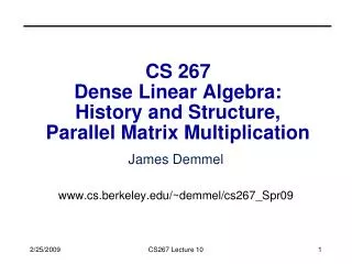
Processor-DRAM Gap (latency) • Memory hierarchies are getting deeper • Processors get faster more quickly than memory µProc 60%/yr. 1000 CPU “Moore’s Law” 100 Processor-Memory Performance Gap:(grows 50% / year) Performance 10 DRAM 7%/yr. DRAM 1 1980 1981 1982 1983 1984 1985 1986 1987 1988 1989 1990 1991 1992 1993 1994 1995 1996 1997 1998 1999 2000 Time CS267 Lecure 2
Approaches to Handling Memory Latency • Bandwidth has improved more than latency • Approach to address the memory latency problem • Eliminate memory operations by saving values in small, fast memory (cache) and reusing them • need temporal locality in program • Take advantage of better bandwidth by getting a chunk of memory and saving it in small fast memory (cache) and using whole chunk • need spatial locality in program • Take advantage of better bandwidth by allowing processor to issue multiple reads to the memory system at once • concurrency in the instruction stream, eg load whole array, as in vector processors; or prefetching CS267 Lecure 2
Cache Basics • Cache hit: in-cache memory access—cheap • Cache miss: non-cached memory access—expensive • Need to access next, slower level of cache • Consider a tiny cache (for illustration only) • Cache line length: # of bytes loaded together in one entry • 2 in above example • Associativity • direct-mapped: only 1 address (line) in a given range in cache • n-way: n 2 lines with different addresses can be stored CS267 Lecure 2
Why Have Multiple Levels of Cache? • On-chip vs. off-chip • On-chip caches are faster, but limited in size • A large cache has delays • Hardware to check longer addresses in cache takes more time • Associativity, which gives a more general set of data in cache, also takes more time • Some examples: • Cray T3E eliminated one cache to speed up misses • IBM uses a level of cache as a “victim cache” which is cheaper • There are other levels of the memory hierarchy • Register, pages (TLB, virtual memory), … • And it isn’t always a hierarchy CS267 Lecure 2
Experimental Study of Memory (Membench) • Microbenchmark for memory system performance • for array A of length L from 4KB to 8MB by 2x • for stride s from 4 Bytes (1 word) to L/2 by 2x • time the following loop • (repeat many times and average) • for i from 0 to L by s • load A[i] from memory (4 Bytes) time the following loop (repeat many times and average) for i from 0 to L by s load A[i] from memory (4 Bytes) CS267 Lecure 2
memory time size > L1 cache hit time total size < L1 Membench: What to Expect average cost per access • Consider the average cost per load • Plot one line for each array length, time vs. stride • Small stride is best: if cache line holds 4 words, at most ¼ miss • If array is smaller than a given cache, all those accesses will hit (after the first run, which is negligible for large enough runs) • Picture assumes only one level of cache • Values have gotten more difficult to measure on modern procs s = stride CS267 Lecure 2
Mem: 396 ns (132 cycles) L2: 2 MB, 12 cycles (36 ns) L1: 16 KB 2 cycles (6ns) L1: 16 B line L2: 64 byte line 8 K pages, 32 TLB entries Memory Hierarchy on a Sun Ultra-2i Sun Ultra-2i, 333 MHz Array length See www.cs.berkeley.edu/~yelick/arvindk/t3d-isca95.ps for details CS267 Lecure 2
Memory Hierarchy on a Pentium III Array size Katmai processor on Millennium, 550 MHz L2: 512 KB 60 ns L1: 64K 5 ns, 4-way? L1: 32 byte line ? CS267 Lecure 2
Mem: 396 ns (132 cycles) L2: 8 MB 128 B line 9 cycles L1: 32 KB 128B line .5-2 cycles Memory Hierarchy on a Power3 (Seaborg) Power3, 375 MHz Array size CS267 Lecure 2
Memory Performance on Itanium 2 (CITRIS) Itanium2, 900 MHz Array size Mem: 11-60 cycles L3: 2 MB 128 B line 3-20 cycles L2: 256 KB 128 B line .5-4 cycles L1: 32 KB 64B line .34-1 cycles Uses MAPS Benchmark: http://www.sdsc.edu/PMaC/MAPs/maps.html CS267 Lecure 2
Lessons • Actual performance of a simple program can be a complicated function of the architecture • Slight changes in the architecture or program change the performance significantly • To write fast programs, need to consider architecture • True on sequential or parallel processor • We would like simple models to help us design efficient algorithms • We will illustrate with a common technique for improving cache performance, called blocking or tiling • Idea: used divide-and-conquer to define a problem that fits in register/L1-cache/L2-cache CS267 Lecure 2
Outline • Idealized and actual costs in modern processors • Memory hierarchies • Case Study: Matrix Multiplication • Automatic Performance Tuning CS267 Lecure 2
Why Matrix Multiplication? • An important kernel in scientific problems • Appears in many linear algebra algorithms • Closely related to other algorithms, e.g., transitive closure on a graph using Floyd-Warshall • Optimization ideas can be used in other problems • The best case for optimization payoffs • The most-studied algorithm in high performance computing CS267 Lecure 2
Matrix-multiply, optimized several ways Speed of n-by-n matrix multiply on Sun Ultra-1/170, peak = 330 MFlops CS267 Lecure 2
Outline • Idealized and actual costs in modern processors • Memory hierarchies • Case Study: Matrix Multiplication • Simple cache model • Warm-up: Matrix-vector multiplication • Blocking algorithms • Other techniques • Automatic Performance Tuning CS267 Lecure 2
Note on Matrix Storage • A matrix is a 2-D array of elements, but memory addresses are “1-D” • Conventions for matrix layout • by column, or “column major” (Fortran default); A(i,j) at A+i+j*n • by row, or “row major” (C default) A(i,j) at A+i*n+j • recursive (later) • Column major (for now) Column major matrix in memory Row major Column major 0 5 10 15 0 1 2 3 1 6 11 16 4 5 6 7 2 7 12 17 8 9 10 11 3 8 13 18 12 13 14 15 4 9 14 19 16 17 18 19 Blue row of matrix is stored in red cachelines cachelines CS267 Lecure 2 Figure source: Larry Carter, UCSD
Computational Intensity: Key to algorithm efficiency Machine Balance:Key to machine efficiency Using a Simple Model of Memory to Optimize • Assume just 2 levels in the hierarchy, fast and slow • All data initially in slow memory • m = number of memory elements (words) moved between fast and slow memory • tm = time per slow memory operation • f = number of arithmetic operations • tf = time per arithmetic operation << tm • q = f / m average number of flops per slow memory access • Minimum possible time = f* tf when all data in fast memory • Actual time • f * tf + m * tm = f * tf * (1 + tm/tf * 1/q) • Larger q means time closer to minimum f * tf • q tm/tfneeded to get at least half of peak speed CS267 Lecure 2
Warm up: Matrix-vector multiplication {implements y = y + A*x} for i = 1:n for j = 1:n y(i) = y(i) + A(i,j)*x(j) A(i,:) + = * y(i) y(i) x(:) CS267 Lecure 2
Warm up: Matrix-vector multiplication {read x(1:n) into fast memory} {read y(1:n) into fast memory} for i = 1:n {read row i of A into fast memory} for j = 1:n y(i) = y(i) + A(i,j)*x(j) {write y(1:n) back to slow memory} • m = number of slow memory refs = 3n + n2 • f = number of arithmetic operations = 2n2 • q = f / m ~= 2 • Matrix-vector multiplication limited by slow memory speed CS267 Lecure 2
Modeling Matrix-Vector Multiplication • Compute time for nxn = 1000x1000 matrix • Time • f * tf + m * tm = f * tf * (1 + tm/tf * 1/q) • = 2*n2 * tf * (1 + tm/tf * 1/2) • For tf and tm, using data from R. Vuduc’s PhD (pp 351-3) • http://bebop.cs.berkeley.edu/pubs/vuduc2003-dissertation.pdf • For tm use minimum-memory-latency / words-per-cache-line machine balance (q must be at least this for ½ peak speed) CS267 Lecure 2
Simplifying Assumptions • What simplifying assumptions did we make in this analysis? • Ignored parallelism in processor between memory and arithmetic within the processor • Sometimes drop arithmetic term in this type of analysis • Assumed fast memory was large enough to hold three vectors • Reasonable if we are talking about any level of cache • Not if we are talking about registers (~32 words) • Assumed the cost of a fast memory access is 0 • Reasonable if we are talking about registers • Not necessarily if we are talking about cache (1-2 cycles for L1) • Memory latency is constant • Could simplify even further by ignoring memory operations in X and Y vectors • Mflop rate/element = 2 / (2* tf + tm) CS267 Lecure 2
Validating the Model • How well does the model predict actual performance? • Actual DGEMV: Most highly optimized code for the platform • Model sufficient to compare across machines • But under-predicting on most recent ones due to latency estimate CS267 Lecure 2
Naïve Matrix Multiply {implements C = C + A*B} for i = 1 to n for j = 1 to n for k = 1 to n C(i,j) = C(i,j) + A(i,k) * B(k,j) Algorithm has 2*n3 = O(n3) Flops and operates on 3*n2 words of memory q potentially as large as 2*n3 / 3*n2 = O(n) A(i,:) C(i,j) C(i,j) B(:,j) = + * CS267 Lecure 2
Naïve Matrix Multiply {implements C = C + A*B} for i = 1 to n {read row i of A into fast memory} for j = 1 to n {read C(i,j) into fast memory} {read column j of B into fast memory} for k = 1 to n C(i,j) = C(i,j) + A(i,k) * B(k,j) {write C(i,j) back to slow memory} A(i,:) C(i,j) C(i,j) B(:,j) = + * CS267 Lecure 2
Naïve Matrix Multiply Number of slow memory references on unblocked matrix multiply m = n3 to read each column of B n times + n2 to read each row of A once + 2n2 to read and write each element of C once = n3 + 3n2 So q = f / m = 2n3 / (n3 + 3n2) ~= 2 for large n, no improvement over matrix-vector multiply A(i,:) C(i,j) C(i,j) B(:,j) = + * CS267 Lecure 2
Matrix-multiply, optimized several ways Speed of n-by-n matrix multiply on Sun Ultra-1/170, peak = 330 MFlops CS267 Lecure 2
Naïve Matrix Multiply on RS/6000 12000 would take 1095 years T = N4.7 Size 2000 took 5 days O(N3) performance would have constant cycles/flop Performance looks like O(N4.7) CS267 Lecure 2 Slide source: Larry Carter, UCSD
Naïve Matrix Multiply on RS/6000 Page miss every iteration TLB miss every iteration Cache miss every 16 iterations Page miss every 512 iterations CS267 Lecure 2 Slide source: Larry Carter, UCSD
Blocked (Tiled) Matrix Multiply Consider A,B,C to be N-by-N matrices of b-by-b subblocks where b=n / N is called the block size for i = 1 to N for j = 1 to N {read block C(i,j) into fast memory} for k = 1 to N {read block A(i,k) into fast memory} {read block B(k,j) into fast memory} C(i,j) = C(i,j) + A(i,k) * B(k,j) {do a matrix multiply on blocks} {write block C(i,j) back to slow memory} A(i,k) C(i,j) C(i,j) = + * B(k,j) CS267 Lecure 2
Blocked (Tiled) Matrix Multiply Recall: m is amount memory traffic between slow and fast memory matrix has nxn elements, and NxN blocks each of size bxb f is number of floating point operations, 2n3 for this problem q = f / m is our measure of algorithm efficiency in the memory system So: m = N*n2 read each block of B N3 times (N3 * b2 = N3 * (n/N)2 = N*n2) + N*n2 read each block of A N3 times + 2n2 read and write each block of C once = (2N + 2) * n2 So computational intensity q = f / m = 2n3 / ((2N + 2) * n2) ~= n / N = b for large n So we can improve performance by increasing the blocksize b Can be much faster than matrix-vector multiply (q=2) CS267 Lecure 2
Using Analysis to Understand Machines The blocked algorithm has computational intensity q ~= b • The larger the block size, the more efficient our algorithm will be • Limit: All three blocks from A,B,C must fit in fast memory (cache), so we cannot make these blocks arbitrarily large • Assume your fast memory has size Mfast 3b2 <= Mfast, so q ~= b <= sqrt(Mfast/3) • To build a machine to run matrix multiply at 1/2 peak arithmetic speed of the machine, we need a fast memory of size Mfast >= 3b2 ~= 3q2 = 3(tm/tf)2 • This size is reasonable for L1 cache, but not for register sets • Note: analysis assumes it is possible to schedule the instructions perfectly CS267 Lecure 2
Limits to Optimizing Matrix Multiply • The blocked algorithm changes the order in which values are accumulated into each C[i,j] by applying associativity • Get slightly different answers from naïve code, because of roundoff - OK • The previous analysis showed that the blocked algorithm has computational intensity: q ~= b <= sqrt(Mfast/3) • There is a lower bound result that says we cannot do any better than this (using only associativity) • Theorem (Hong & Kung, 1981): Any reorganization of this algorithm (that uses only associativity) is limited to q = O(sqrt(Mfast)) • What if more levels of memory hierarchy? • Apply blocking recursively, once per level CS267 Lecure 2
Basic Linear Algebra Subroutines (BLAS) • Industry standard interface (evolving) • www.netlib.org/blas, www.netlib.org/blas/blast--forum • Vendors, others supply optimized implementations • History • BLAS1 (1970s): • vector operations: dot product, saxpy (y=a*x+y), etc • m=2*n, f=2*n, q ~1 or less • BLAS2 (mid 1980s) • matrix-vector operations: matrix vector multiply, etc • m=n^2, f=2*n^2, q~2, less overhead • somewhat faster than BLAS1 • BLAS3 (late 1980s) • matrix-matrix operations: matrix matrix multiply, etc • m <= 3n^2, f=O(n^3), so q=f/m can possibly be as large as n, so BLAS3 is potentially much faster than BLAS2 • Good algorithms used BLAS3 when possible (LAPACK & ScaLAPACK) • Seewww.netlib.org/{lapack,scalapack} • More later in course CS267 Lecure 2
BLAS speeds on an IBM RS6000/590 Peak speed = 266 Mflops Peak BLAS 3 BLAS 2 BLAS 1 BLAS 3 (n-by-n matrix matrix multiply) vs BLAS 2 (n-by-n matrix vector multiply) vs BLAS 1 (saxpy of n vectors) CS267 Lecure 2
Strassen’s Matrix Multiply • The traditional algorithm (with or without tiling) has O(n^3) flops • Strassen discovered an algorithm with asymptotically lower flops • O(n^2.81) • Consider a 2x2 matrix multiply, normally takes 8 multiplies, 4 adds • Strassen does it with 7 multiplies and 18 adds Let M = m11 m12 = a11 a12 b11 b12 m21 m22 = a21 a22 b21 b22 Let p1 = (a12 - a22) * (b21 + b22) p5 = a11 * (b12 - b22) p2 = (a11 + a22) * (b11 + b22) p6 = a22 * (b21 - b11) p3 = (a11 - a21) * (b11 + b12) p7 = (a21 + a22) * b11 p4 = (a11 + a12) * b22 Then m11 = p1 + p2 - p4 + p6 m12 = p4 + p5 m21 = p6 + p7 m22 = p2 - p3 + p5 - p7 Extends to nxn by divide&conquer CS267 Lecure 2
Strassen (continued) • Asymptotically faster • Several times faster for large n in practice • Cross-over depends on machine • Available in several libraries • “Tuning Strassen's Matrix Multiplication for Memory Efficiency”, M. S. Thottethodi, S. Chatterjee, and A. Lebeck, in Proceedings of Supercomputing '98 • Caveats • Needs more memory than standard algorithm • Can be less accurate because of roundoff error CS267 Lecure 2
Other Fast Matrix Multiplication Algorithms • Current world’s record is O(n 2.376... ) (Coppersmith & Winograd) • Why does Hong/Kung theorem not apply? • Possibility of O(n2+) algorithm! (Cohn, Umans, Kleinberg, 2003) • Fast methods (besides Strassen) may need unrealistically large n CS267 Lecure 2
Recursive Data Layouts • Blocking seems to require knowing cache sizes – portable? • A related (recent) idea is to use a recursive structure for the matrix • There are several possible recursive decompositions depending on the order of the sub-blocks • This figure shows Z-Morton Ordering (“space filling curve”) • See papers on “cache oblivious algorithms” and “recursive layouts” • Will be in next LAPACK release (Gustavson, Kagstrom, et al, SIAM Review, 2004) • Advantages: • the recursive layout works well for any cache size • Disadvantages: • The index calculations to find A[i,j] are expensive • Implementations switch to column-major for small sizes CS267 Lecure 2
Outline • Idealized and actual costs in modern processors • Memory hierarchies • Case Study: Matrix Multiplication • Automatic Performance Tuning (see next file) CS267 Lecure 2
Extra Slides CS267 Lecure 2
Search Over Block Sizes • Performance models are useful for high level algorithms • Helps in developing a blocked algorithm • Models have not proven very useful for block size selection • too complicated to be useful • See work by Sid Chatterjee for detailed model • too simple to be accurate • Multiple multidimensional arrays, virtual memory, etc. • Speed depends on matrix dimensions, details of code, compiler, processor • Some systems use search over “design space” of possible implementations • Atlas – incorporated into Matlab • BeBOP – http://www.cs.berkeley.edu/~richie/bebop CS267 Lecure 2