Solution Manual for Feedback Systems 2nd Edition by Astrom and Murray

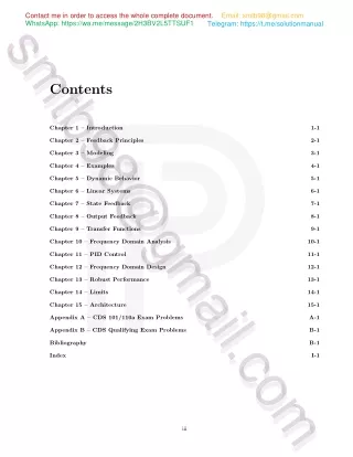
1. Email: smtb98@gmail.com Telegram: https://t.me/solutionmanual Contact me in order to access the whole complete document. WhatsApp: https://wa.me/message/2H3BV2L5TTSUF1 smtb98@gmail.com smtb98@gmail.com Contents Chapter 1 – Introduction 1-1 Chapter 2 – Feedback Principles 2-1 Chapter 3 – Modeling 3-1 Chapter 4 – Examples 4-1 Chapter 5 – Dynamic Behavior 5-1 Chapter 6 – Linear Systems 6-1 Chapter 7 – State Feedback 7-1 Chapter 8 – Output Feedback 8-1 Chapter 9 – Transfer Functions 9-1 Chapter 10 – Frequency Domain Analysis 10-1 Chapter 11 – PID Control 11-1 Chapter 12 – Frequency Domain Design 12-1 Chapter 13 – Robust Performance 13-1 Chapter 14 – Limits 14-1 Chapter 15 – Architecture 15-1 Appendix A – CDS 101/110a Exam Problems A-1 Appendix B – CDS Qualifying Exam Problems B-1 Bibliography B-1 Index I-1 iii

2. Email: smtb98@gmail.com Telegram: https://t.me/solutionmanual Contact me in order to access the whole complete document. WhatsApp: https://wa.me/message/2H3BV2L5TTSUF1 Chapter 1 – Introduction 1-1 Chapter 1 – Introduction 1.1 Identify five feedback systems that you encounter in your everyday environment. For each system, identify the sensing mechanism, actuation mechanism, and control law. respect to which the feedback system provides robustness and/or the dynamics that are changed through the use of feedback. Describe the uncertainty with Instructor note: The main point of this problem is to get students to think about what a feedback/control system is and what the different elements are. Solution. Some sample answers are provided below. Air Conditioning • Sensing: A thermal sensor detects the ambient temperature of the room. • Computation: Internal logic compares the ambient temperature to the temperature set on the dial. • Actuation: A fan and compressor deliver cold air to cool off the room. • Effect: A desired temperature is maintained despite uncertainty of other heat inputs (like sunlight). Washing Machine • Sensing: A mechanical sensor reports the rotational speed of the drum. • Computation: The current speed is compared to the desired speed for a particular laundry setting. • Actuation: The electrical motor drives the rotation of the drum. • Effect: A desired rotational speed is maintained despite variations in laundry load. Human Locomotion • Sensing: Eyes and various internal balance mechanisms report the environment and the current motion of the body. • Computation: The brain maintains several feedback loops between motion, environment, and desired destination. • Actuation: Muscles move limbs in periodic trajectories. • Effect: Walking is accomplished in dynamic and uncertain environments (like hills, stairs). 1.2 (Balance systems) Balance yourself on one foot with your eyes closed for 15 s. Using Figure 1.4 as a guide, describe the control system responsible for keeping you from falling down. Note that the “controller” will differ from that in the diagram (unless you are an android reading this in the far future). Solution. [Cole Lepine, Feb 08] We will describe each part of the control system using the labels of Figure 1.4. We also remove the Filter, A/D, D/A, and Clock labels because they do not apply to a human body. Noise: This is the noise that enters the system between the computer and the actuators. For the human body, this could be noise that enters along the neural pathway, due to the stochastic nature of neural signaling. Actuators: The actuators for the human body are the muscles. For this problem of keeping balance, you use the muscles in your feet and possibly the motion of your arms. System: The system is your body balanced on top of your legs and feet. Its dynamics obey the usual laws of physics. External Disturbances: This would be anything that effects the system that we do not have control over, like air currents or the stability of the ground. Sensors: The sensors of the human body for this problem is the fluid in your inner ear, and your sense of touch on the ground. complete document is available on https://solumanu.com/ *** contact me if site not loaded

3. Email: smtb98@gmail.com Telegram: https://t.me/solutionmanual Contact me in order to access the whole complete document. WhatsApp: https://wa.me/message/2H3BV2L5TTSUF1 Computer: The human brain that processes the signals generated by your body and sends out the commands to correct for any balance problems. smtb98@gmail.com Noise: This is the noise that enters the system as a result of the sensing process. For the human body, this could be the noise that enters along the neural pathway from the senses to the computer, or from imperfections in the sensing equipment (like diseases effecting your inner ear or your sense of touch). smtb98@gmail.com 1-2 Feedback Systems: Solutions Manual - v2.2a Operator Input: The human will. Maybe you want to fall down! ? 1.3 (Eye motion) Perform the following experiment and explain your results: Holding your head still, move one of your hands left and right in front of your face, following it with your eyes. Record how quickly you can move your hand before you begin to lose track of it. Now hold your hand still and shake your head left to right, once again recording how quickly you can move before losing track of your hand. Explain any difference in performance by comparing the control systems used to implement these behaviors. Solution. The eye along with its vision system is one of the few organs that is easily accessible to experiments. An initial thought about this experiment is that it would be easier to track fast if the head is fixed and only the eyes move, simply because the head has a much larger moment of inertia than the eye. The experiment shows that this is not true. The reason is due to the properties of the feedback systems. When the head is moved there are gyroscopic sensors for angular rate that sends signals directly to the eyes to keep the line of sight constant. When the head is kept fixed and the eyes are moving the information about the image has to be processed in the brain before signals can be sent to the eyes to move them. This signal processing takes some time which explains why tracking is slower in this case. 1.4 (Cruise control) Download the MATLAB code used to produce simulations for the cruise control system in Figure 1.11 from the companion web site. Using trial and error, change the parameters of the control law so that the overshoot in speed is not more than 1 m/s for a vehicle with mass m = 1200 kg. Does the same controller work if we set m = 2000 kg? Solution. [Cole Lepine, Feb 08] Although there are more than one set of parameters that work, here are ones that do: kp= 2 and ki= 0.1. Figure S1.1 shows a graph of how the system responds to a change in 32 30 28 Speed v [m/s] 26 24 22 20 18 0 20 40 60 Time t [s] Figure S1.1: Step response for the redesigned cruise control system in Exercise 1.4. This shows that the overshoot is less than 1 m/s for the given gains. reference speed from 20 m/s to 30 m/s at t = 20 s. The MATLAB code used to generate the plot is plot(Time, Vel); xlabel(’time (sec)’); ylabel(’speed (m/s)’); (to be used after running the SIMULINK model). 1.5 (Integral action) We say that a system with a constant input reaches steady state if all system variables approach constant values as time increases. Show that a controller with integral action, such as those given in equations (1.4) and (1.5), gives zero error if the closed loop system reaches steady state. Notice that there is no saturation in the controller. complete document is available on https://solumanu.com/ *** contact me if site not loaded

4. Chapter 1 – Introduction 1-3 Instructor note: This exercise is worked out in Section 11.1. Solution. Consider the controller given by equation (1.5). Assume that there exist a steady state with u = u0 and e = e0. It then follows from equation (1.5) that u0= kpe0+ kie0t, which is a contradiction unless e0or kiis zero. We can thus conclude that with integral action the error will be zero if there is a steady state. Notice that we have not made any assumptions about linearity of the process or the disturbances. We have, however assumed that an equilibrium point exists. Using integral action to achieve zero steady-state error is much better than using feedforward, which requires precise knowledge of process parameters. 1.6 (Combining feedback with logic) Consider a system for cruise control where the overall function is governed by the state machine in Figure 1.16. Assume that the system has a continuous input for vehicle velocity, discrete inputs indicating braking and gear changes, and a PI controller with inputs for the reference and measured velocities and an output for the control signal. Sketch the actions that have to be taken in the states of the finite state machine to handle the system properly. Think about if you have to store some extra variables, and if the PI controller has to be modified. Solution. Because the cruise control system is expected to remember that last reference speed that it was set for, an extra variable is required to keep track of this reference value and set it properly. Letting ref represent the desired speed of the vehicle, the following actions should be taken in the states and transitions of the finite state machine: • Standby → Cruise via the Set action: set the value of ref to the current speed. • Cruise mode: if Coast/Set is pressed, decrease the value of ref; if Res/Accel is pressed, increase the value of ref. In addition, because the controller has an integrator, the controller requires a variable to keep track of the ? integrated error up to the current time. This variable has to be initialized properly to ensure that it does not create undesireable control actions when the system switches modes. This is called the “bumpless transfer” problem and is mentioned briefly in Section 13.4. 1.7 Search the web and pick an article in the popular press about a feedback and control system. Describe the feedback system using the terminology given in the article. In particular, identify the control system and describe (a) the underlying process or system being controlled, along with the (b) sensor, (c) actuator, and (d) computational element. If the some of the information is not available in the article, indicate this and take a guess at what might have been used. Instructor note: The goal of this exercise is to have students read a bit about popular descriptions of control systems and relate this to the terminology in Chapter 1. Solution. A sample answer is provided below. Anti-Rollover Technology: The US Government has proposed that anti-rollover technology be required for all new vehicles by the year 2012. The following web sites contain information on the required technology: • NHTSA press release: http://www.nhtsa.dot.gov → Press Releases → 2006 → “DOT Proposes Anti-Rollover Technology for New Vehicles” • Electronic stability control overview: http://www.safercar.gov → Rollover → Electronic Stability Control Based on the information presented on these web sites, the control system has the following components: (a) Process: vehicle dynamics as it drives, including dynamics associated with acceleration, braking, and sliding complete document is available on https://solumanu.com/ *** contact me if site not loaded

5. (d) Computation: If the yaw rate of the car is greater than what is expected from the current steering position and velocity of the car, we are in a spin out, and we should actuate the outside front brake. If the reverse is true (the yaw rate of the car is less than expected) the car is plowing out, and we must actuate the rear inner brake. smtb98@gmail.com (b) Sensing: Steering wheel position sensor; yaw-rate sensor (accelerometer) smtb98@gmail.com 1-4 Feedback Systems: Solutions Manual - v2.2a (c) Actuation: Individual braking of wheels Supplemental Exercises 1.8 Make a schematic picture of the system for supplying milk from a cow to your table. Discuss the impact of refrigerated storage. Solution. A schematic picture of the system is shown in the figure below. Since the quality of milk deteriorates with time, it is necessary to have a short delay between milking and consumption. Before refrigeration it was necessary to have production and consumption in close proximity. When refrigeration and pasteurization were introduce it was possible to introduce large diaries and distribution that covers large areas. When the direct link between producers and consumers was broken it was necessary to introduce feedback links in the system (indicated by dashed lines in the figure) to maintain balance between production and consumption. 1.9 (MATLAB/SIMULINK) Download the file “cruise_ctrl.mdl” from the companion web site. It con- tains a SIMULINK model of a simple cruise controller, similar to the one described in Section 1.5. Figure out how to run the example and plot the vehicle’s speed as a function of time. (a) Leaving the control gains at their default values, plot the response of the system to a step input and measure the time it takes for the system error to settle to within 5% of commanded change in speed (i.e., 0.5 m/s). (b) By manually tuning the control gains, design a controller that settles at least 50% faster than the default controller. Include the gains you used, a plot of the closed loop response, and describe any undesirable features in the solution you obtain. All plots should included a title, labeled axes (with units), and reasonable axis limits. Instructor note: The exercise is a variation of Exercise 1.4 above. The purpose of these problem is to give students some familiarity with MATLAB and SIMULINK. The instructor may want to indicate in the problem that students shouldn’t worry if they don’t yet know how the control law works or why it does what it does. Solution. [Caltech CDS 101/110 TAs, 2004–2006; Cole Lepine, Feb 08] (a) The red curve in Figure S1.2 depicts speed as a function of time for the default gains. It was created by first running the simulation, then in the MATLAB command window running the command: plot(Time, Vel); xlabel(’time (sec)’); ylabel(’speed (m/s)’); We calculate the settling time by finding the first time after which the system remains within the five percent bound specified. This occurs at about 34 second and can be found after running the simulation with the commands: settle = find (abs(flipud(Vel) - 30) > .5); timerev = flipud(Time); timerev(settle(1)); This searches through the velocity vector backwards to find the first out of bounds value, and then computes the time at which that point occurs. Finally we subtract the time at which the system input began, i.e. t = 20 s, and obtain a settling time of 14 s. complete document is available on https://solumanu.com/ *** contact me if site not loaded

6. Chapter 1 – Introduction 1-5 35 30 Speed v [m/s] 25 20 15 0 20 40 60 Time t [s] Figure S1.2: Response of cruise control system to step input. The red curve shows the response using original controller gains for Exercise ??. This shows that the settling time is about 15 s for the given gains. The blue curve show the modified gains, which give a settling time is about 7 s. (b) We want to modify the control parameters so that the system settles 50% faster, or within 7 s. In this example, increasing the proportional gain resulted in faster, sharper response. Increasing the integral gain does not have much effect on the responsiveness of the system, and for sufficiently large values induces oscillatory behavior, which is undesirable. A choice of gains that accomplishes the desired behavior is ki = 0.1 and kp = 3.3. This has a settling time (calculated as above) of 7 s. The blue curve in Figure S1.2 shows the system response for these gains. With the exception of the fact that this performance may be difficult to achieve in reality due to the constraints discussed below, there are no undersirable features of the new response as compared to the default performance. Of course, we can increase the proportional gain even further, and obtain a faster response time. Extremely large values could result in extremely fast response. This control strategy is limited by physical realism: there’s only so much power an engine can provide, only so much traction on any given surface, and only so much acceleration that a passenger (or designer) will tolerate. Certainly, attempting a 10 m/s increase in speed in under a second is an ambitious undertaking, even though it is easy enough to dial up kpsufficiently in order to achieve this within our simple model. 1.10 (MATLAB/SIMULINK) Download the file “ballbeam.mdl” from the companion web site. It contains a SIMULINK model of a “ball and beam” experiment in which you apply a torque to a beam and try to balance a ball that rolls along the beam (see course web page for more documentation). (a) Run the simulation with default parameters and create a plot of the ball position versus time. Note that the desired action of the system is to move the ball from its initial position at the center of the beam to a new resting point at r = 0.25 m. (b) While keeping the gain on ˙ α fixed at its default value, vary the gain on α from 75% to three times the default value. Plot the “overshoot” (the maximum amount by which the ball goes past the desired resting point, expressed as a percentage of the commanded position) as a function of this gain for stable cases. (c) While keeping gain on α fixed at its default value, vary the gain on ˙ α from zero to twice its default value. Give the numerical range of this gain for which the system is stable. Plot the “settling time” (amount of time required for the system to get within 5% of the desired resting point) as a function of this gain for the stable cases. All plots should included a title, labeled axes (with units), and reasonable axis limits. Solution. [Lars Cremean, 2003; Steve Waydo, 2006] The solutions make use of the SIMULINK model available on the companion web site. (a) Figure S1.3a depicts the ball position as a function of time for the default gains. It was created by first running the simulation, then in the MATLAB command window running the command:

7. smtb98@gmail.com smtb98@gmail.com 1-6 Feedback Systems: Solutions Manual - v2.2a 0.4 45 7 6 0.3 40 Ball position [m] settling times, s overshoot, % 5 35 4 0.2 30 3 25 2 0.1 20 1 0 0 0 10 20 30 1000 1500 gain on α 2000 100 200 gain on α dot 300 Time [sec] (a) Ball position, default gains (b) Overshoot versus gain (c) Settling time versus gain Figure S1.3: Design trade-offs for the ball and beam system. plot(ballbeam.time, ballbeam.signals.values(:,1)) (b) The system can be seen to be stable for a gain kαon α of at least 730. Figure S1.3b is a plot of the overshoot as a percentage of commanded position as a function of kαfor the default gain k˙ αon ˙ α of 350. (c) The system can be seen to be stable for a gain k˙ αon ˙ α from 80 to 380. Figure S1.3c is a plot of the settling time as a function of k˙ αfor the default kαof 800. MATLAB code: ballbeam_mlintro.m 1.11 Search for the term “voltage clamp” on the Internet and explore why it is so advantageous to use feedback to measure the ion current in cells. You may also enjoy reading about the Nobel Prizes received by Hodgkin and Huxley 1963 and Neher and Sakmann (see http://nobelprizes.org). 1.12 Search for the term “force feedback” and explore its use in haptics and sensing. 1.13 Read the April 2007 Detroit News article “Officials mandate anti-rollover rule” (available from the companion web site). This article talks about new regulations that are being proposed to use anti-rollover technology in cars sold in the U.S. beginning in 2012. By reading the article and the companion articles on the National Highway Traffic Safety Administration (NHTSA) web site, identify the sensing and actuation systems that will be used, and summarize how the control algorithm for the system works. Solution. • Sensing: Steering wheel position sensor; yaw-rate sensor (accelerometer) • Actuation: Individual braking of wheels • Control algorithm: If the yaw rate of the car is greater than what is expected from the current steering position and velocity of the car, we are in a spin out, and we should actuate the outside front brake. If the reverse is true (the yaw rate of the car is less than expected) the car is plowing out, and we must actuate the rear inner brake.

8. Chapter 2 – Feedback Principles 2-1 Chapter 2 – Feedback Principles 2.1 (Transfer functions and differential equations) Let y ∈ R and u ∈ R. Solve the differential equations dy dt+ ay = bu, d2y dt2+ 2dy dt+ y = 2du dt+ u, for t > 0. Determine the responses to a unit step u(t) = 1 and the exponential signal u(t) = estwhen the initial condition is zero. Derive the transfer functions of the systems. Solution. [Contributions from J. Cruz, 2015] first-order equation We will first solve the homogeneous equation dy dt= −ay, hence dy dt= −at, y(t) = e−at+c= e−atC logy = −at + c, To find a particular solution we use the method of variation of the constant, hence assume a solution of the form y(t) = e−atC(t). Inserting this expression in the differential equation gives e−atdC dt− ae−atC = −ae−atC + bu, Hence Zt dC dt = eatbu(t), eaτbu(τ)dτ C(t) = 0 And we find the particular solution Zt Zt y(t) = e−atC(t) = e−at e−a(t−τ)bu(τ)dτ eaτbu(τ)dτ = 0 0 Combining with the he general solution to the homogeneous equation then gives the solution Zt y(t) = e−aty0+ e−a(t−τ)bu(τ)dτ, 0 where y0is a constant. Since y(0) = y0the constant C can be interpreted as the initial condition. The unit step response is the solution corresponding to y0= 0 and u(t) = 1. Zt The response to the exponential signal is the solution corresponding to y0= 0 and u(t) = est: Zt In steady state, the negative exponential goes to zero and so the steady-state response to the complex exponential is s + aest. Dividing by the input we get the transfer function: Zt eaτdτ =b e−a(t−τ)dτ = be−at a(1 − e−at). y(t) = b 0 0 b y(t) = be−at s + a(est− e−at). e(a+s)τdτ = 0 b yss= G(s) =yss b est= s + a

9. A particular solution for the input u(t) = 1 is y(t) = 1, it has two zeros at s = −1. The general solution corresponding to a step input is then smtb98@gmail.com second-order equation The characteristic polynomial is s2+2s+1 = (s+1)2. The general solution to the homogeneous equation smtb98@gmail.com 2-2 Feedback Systems: Solutions Manual - v2.2a is y(t) = Ae−t+ Bte−t. y(t) = 1 + Ae−t+ Bte−t. We have ˙ y = −Ae−t+ Be−t− Bte−t. The initial conditions y(0) = 0 and ˙ y(0) = 0 give −A + B = 0. 1 + A = 0, Hence A = −1 and B = −1. The solution is y(t) = 1 − e−t− te−t. To compute the response to the exponential signal, we use the variation of parameters formula to find a particular solution with forcing function r(t) = (2s+1)est, i.e. the right hand side of the equation evaluated with u = est. With two linearly independent homogeneous solutions given by y1(t) = e−tand y2(t) = te−t, the variation of parameters formula is Zt where W(τ) is the Wronskian. Evaluating the integrals with the data from our problem we get Zt y2(τ)r(τ) W(τ) y1(τ)r(τ) W(τ) yp= −y1(t) dτ + y2(t) dτ 0 0 ?est− e−t− t(1 + s)e−t?. 2s + 1 (s + 1)2 yp= It is easy to check that this solution satisfies the zero initial conditions, and so it is the response to the exponential input. As in the first-order problem, we can simply look at the steady-state behavior and divide by the exponential input to get the transfer function 2s + 1 (s + 1)2 G(s) = Here is another way to find the transfer function: we assume the input is u(t) − estand we look for a solution of the form y(t) = estG(s). We have ˙ u = sestand ˙ y = sestG(s), ¨ y = s2estG(s) Inserting these expressions in the differential equation gives (s2+ 2s + 1)estG(s) = (2s + 1)est, hence 2s + 1 s2+ 2s + 1. G(s) = This expression can also be obtained directly by inspection. 2.2 (Effect of zeros on time responses) Let y0(t) be the response of a system with the transfer function G0(s) to a given input. The transfer function G(s) = (1 + sT)G0(s) has the same zero frequency gain but it has an additional zero at z = −1/T. Let y(t) be the response of the system with the transfer function G(s) and show that y(t) = y0(t) + Tdy0 dt. (S2.1) complete document is available on https://solumanu.com/ *** contact me if site not loaded