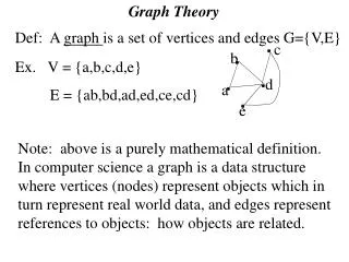
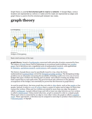
1. Graph theory is used to find shortest path in road or a network. In Google Maps, various locations are represented as vertices or nodes and the roads are represented as edges and graph theory is used to find the shortest path between two nodes. graph theory bridges of Königsberg Read a brief summary of this topic graph theory, branch of mathematics concerned with networks of points connected by lines. The subject of graph theory had its beginnings in recreational math problems (see number game), but it has grown into a significant area of mathematical research, with applications in chemistry, operations research, social sciences, and computer science. The history of graph theory may be specifically traced to 1735, when the Swiss mathematician Leonhard Euler solved the Königsberg bridge problem. The Königsberg bridge problem was an old puzzle concerning the possibility of finding a path over every one of seven bridges that span a forked river flowing past an island—but without crossing any bridge twice. Euler argued that no such path exists. His proof involved only references to the physical arrangement of the bridges, but essentially he proved the first theorem in graph theory. As used in graph theory, the term graph does not refer to data charts, such as line graphs or bar graphs. Instead, it refers to a set of vertices (that is, points or nodes) and of edges (or lines) that connect the vertices. When any two vertices are joined by more than one edge, the graph is called a multigraph. A graph without loops and with at most one edge between any two vertices is called a simple graph. Unless stated otherwise, graph is assumed to refer to a simple graph. When each vertex is connected by an edge to every other vertex, the graph is called a complete graph. When appropriate, a direction may be assigned to each edge to produce what is known as a directed graph, or digraph.

2. In 1857 the Irish mathematician William Rowan Hamilton invented a puzzle (the Icosian Game) that he later sold to a game manufacturer for £25. The puzzle involved finding a special type of path, later known as a Hamiltonian circuit, along the edges of a dodecahedron (a Platonic solid consisting of 12 pentagonal faces) that begins and ends at the same corner while passing through each corner exactly once. The knight’s tour (see number game: Chessboard problems) is another example of a recreational problem involving a Hamiltonian circuit. Hamiltonian graphs have been more challenging to characterize than Eulerian graphs, since the necessary and sufficient conditions for the existence of a Hamiltonian circuit in a connected graph are still unknown.

3. The histories of graph theory and topology are closely related, and the two areas share many common problems and techniques. Euler referred to his work on the Königsberg bridge problem as an example of geometria situs—the “geometry of position”—while the development of topological ideas during the second half of the 19th century became known as analysis situs—the “analysis of position.” In 1750 Euler discovered the polyhedral formula V–E + F = 2 relating the number of vertices (V), edges (E), and faces (F) of a polyhedron (a solid, like the dodecahedron mentioned above, whose faces are polygons). The vertices and edges of a polyhedron form a graph on its surface, and this notion led to consideration of graphs on other surfaces such as a torus (the surface of a solid doughnut) and how they divide the surface into disklike faces. Euler’s formula was soon generalized to surfaces as V–E + F = 2 – 2g, where gdenotes the genus, or number of “doughnut holes,” of the surface (see Euler characteristic). Having considered a surface divided into polygons by an embedded graph, mathematicians began to study ways of constructing surfaces, and later more general spaces, by pasting polygons together. This was the beginning of the field of combinatorial topology, which later, through the work of the French mathematician Henri Poincaré and others, grew into what is known as algebraic topology. The connection between graph theory and topology led to a subfield called topological graph theory. An important problem in this area concerns planar graphs. These are graphs that can be drawn as dot-and- line diagrams on a plane (or, equivalently, on a sphere) without any edges crossing except at the vertices where they meet. Complete graphs with four or fewer vertices are planar, but complete graphs with five vertices (K5) or more are not. Nonplanar graphs cannot be drawn on a plane or on the surface of a sphere without edges intersecting each other between the vertices. The use of diagrams of dots and lines to represent graphs actually grew out of 19th-century chemistry, where lettered vertices denoted individual atoms and connecting lines denoted chemical bonds (with degree corresponding to valence), in which planarity had important chemical consequences. The first use, in this context, of the word graph is attributed to the 19th-century Englishman James Sylvester, one of several mathematicians interested in counting special types of diagrams representing molecules.

4. planar graph and nonplanar graph compared With fewer than five vertices in a two-dimensional plane, a collection of paths between vertices can be drawn in the plane such that no paths intersect. With five or more vertices in a two-dimensional plane, a collection of nonintersecting paths between vertices cannot be drawn without the use of a third dimension. Encyclopædia Britannica, Inc. Another class of graphs is the collection of the complete bipartite graphs Km,n, which consist of the simple graphs that can be partitioned into two independent sets of m and n vertices such that there are no edges between vertices within each set and every vertex in one set is connected by an edge to every vertex in the other set. Like K5, the bipartite graph K3,3 is not planar, disproving a claim made in 1913 by the English recreational problemist Henry Dudeney to a solution to the “gas-water-electricity” problem. In 1930 the Polish mathematician Kazimierz Kuratowski proved that any nonplanar graph must contain a certain type of copy of K5 or K3,3. While K5 and K3,3 cannot be embedded in a sphere, they can be embedded in a torus. The graph-embedding problem concerns the determination of surfaces in which a graph can be embedded and thereby generalizes the planarity problem. It was not until the late 1960s that the embedding problem for the complete graphs Kn was solved for all n.

5. Dudeney puzzle The English recreational problemist Henry Dudeney claimed to have a solution to a problem that he posed in 1913 that required each of three houses to be connected to three separate utilities such that no utility service pipes intersected. Dudeney's solution involved running a pipe through one of the houses, which would not be considered a valid solution in graph theory. In a two-dimensional plane, a collection of six vertices (shown here as the vertices in the homes and utilities) that can be split into two completely separate sets of three vertices (that is, the vertices in the three homes and the vertices in the three utilities) is designated a K3,3 bipartite graph. The two parts of such graphs cannot be interconnected within the two-dimensional plane without intersecting some paths. Encyclopædia Britannica, Inc. Another problem of topological graph theory is the map-colouring problem. This problem is an outgrowth of the well-known four-colour map problem, which asks whether the countries on every map can be coloured by using just four colours in such a way that countries sharing an edge have different colours. Asked originally in the 1850s by Francis Guthrie, then a student at University College London, this problem has a rich history filled with incorrect attempts at its solution. In an equivalent graph-theoretic form, one may translate this problem to ask whether the vertices of a planar graph can always be coloured by using just four colours in such a way that vertices joined by an edge have different colours. The result was finally proved in 1976 by using computerized checking of nearly 2,000 special configurations. Interestingly, the corresponding colouring problem concerning the number of colours required to colour maps on surfaces of higher genus was completely solved a few years earlier; for example, maps on a torus may require as many as seven colours. This work confirmed that a formula of the English mathematician Percy Heawood from 1890 correctly gives these colouringnumbers for all surfaces except the one-sided surface known as the Klein bottle, for which the correct colouring number had been determined in 1934 In the rain-soaked Indian state of Meghalaya, locals train the fast-growing trees to grow over rivers, turning the trees into living bridges. See All Good Facts Among the current interests in graph theory are problems concerning efficient algorithms for finding optimal paths (depending on different criteria) in graphs. Two well-known examples are the Chinese postman problem (the shortest path that visits each edge at least once), which was solved in the 1960s, and the traveling salesman problem (the shortest path that begins and ends at the same vertex and visits each edge exactly once), which continues to attract the attention of many researchers because of its applications in routing data, products, and people. Work on such problems is related to the field of linear programming, which was founded in the mid-20th century by the American mathematician George Dantzig

6. What is Graph Theory, and why should you care? From graph theory to path optimization A graph visualization issued from the Opte Project, a tentative cartography of the Internet Graph theory might sound like an intimidating and abstract topic to you, so why should you even spend your time reading an article about it? However, although it might not sound very applicable, there are actually an abundance of useful and important applications of graph theory! In this article, I will try to explain briefly what some of these applications are. In doing so, I will do my best to convince you that having at least some basic knowledge of this topic can be useful in solving some interesting problems you might come across. In this article, I will through a concrete example show how a route planning/optimization task can be formulated and solved using graph theory. More specifically, I will consider a large warehouse consisting of 1000s of different items in various locations/pickup points. The challenge here is, given a list of items, which path should you follow through the warehouse to pickup all items, but at the same time minimize the total distance traveled? For those of you familiar with these kind of problems, this has quite some resemblance to the famous traveling salesman problem. (A well known problem in combinatorial optimization, important in theoretical computer science and operations research). As you might have realized, the goal of this article is not to give a comprehensive introduction to graph theory (which would be quite a tremendous task). Through a real-world example, I will rather try to convince you that knowing at least some basics of graph theory can prove to be very useful! I will start with a brief historical introduction to the field of graph theory, and highlight the importance and the wide range of useful applications in many vastly different fields. Following

7. this more general introduction, I will then shift focus to the warehouse optimization example discussed above. The history of Graph Theory The basic idea of graphs were first introduced in the 18th century by the Swiss mathematician Leonhard Euler, one of the most eminent mathematicians of the 18th century (and of all time, really). His work on the famous “Seven Bridges of Königsberg problem”, are commonly quoted as origin of graph theory. The city of Königsberg in Prussia (now Kaliningrad, Russia) was set on both sides of the Pregel River, and included two large islands — Kneiphof and Lomse — which were connected to each other, or to the two mainland portions of the city, by seven bridges (as illustrated in the below figure to the left). The problem was to devise a walk through the city that would cross each of those bridges once and only once. Euler, recognizing that the relevant constraints were the four bodies of land & the seven bridges, drew out the first known visual representation of a modern graph. A modern graph, as seen in bottom-right image, is represented by a set of points, known as vertices or nodes, connected by a set of lines known as edges. Credit: Wikipedia This abstraction from a concrete problem concerning a city and bridges etc. to a graph makes the problem tractable mathematically, as this abstract representation includes only the information important for solving the problem. Euler actually proved that this specific problem has no solution. However, the difficulty he faced was the development of a suitable technique of analysis, and of subsequent tests that established this assertion with mathematical rigor. From there, the branch of math known as graph theory lay dormant for decades. In modern times, however, it’s applications are finally exploding. Introduction to Graph Theory As mentioned previously, I do not aim to give a comprehensive introduction to graph theory. The following section still contains some of the basics when it comes to different kind of graphs etc., which is of relevance to the example we will discuss later on path optimization. Graph Theory is ultimately the study of relationships. Given a set of nodes & connections, which can abstract anything from city layouts to computer data, graph theory provides a helpful tool to quantify & simplify the many moving parts of dynamic systems. Studying graphs through

8. a framework provides answers to many arrangement, networking, optimization, matching and operational problems. Graphs can be used to model many types of relations and processes in physical, biological, social and information systems, and has a wide range of useful applications such as e.g. 1.Finding communities in networks, such as social media (friend/connection recommendations), or in the recent days for possible spread of COVID19 in the community through contacts. 2.Ranking/ordering hyperlinks in search engines. 3.GPS/Google maps to find the shortest path home. 4.Study of molecules and atoms in chemistry. 5.DNA sequencing 6.Computer network security 7.….. and many more…. A simple example of a graph with 6 nodes A simple example of a graph with 6 nodes A slightly more complex social media network. Credit: Martin Grandjean Wikimedia

9. As mentioned, there are several types of graphs that describe different kind of problems (and the constraints within them). A nice walk-through of various types of graphs can also be found in a Error! Hyperlink reference not valid. by Kelvin Jose, and the below section represents a subset of that article. Types of Graphs There are different types of graph representations available and we have to make sure that we understand the kind of graph we are working with when programmatically solving a problem which includes graphs. Undirected Graphs • As the name shows, there won’t be any specified directions between nodes. So an edge from node A to B would be identical to the edge from B to A. In the above graph, each node could represent different cities and the edges show the bidirectional roads. Directed Graphs (DiGraphs) • Unlike undirected graphs, directed graphs have orientation or direction among different nodes. That means if you have an edge from node A to B, you can move only from A to B. Credit: WIkiMedia Like the previous example, if we consider nodes as cities, we have a direction from city 1 to 2. That means, you can drive from city 1 to 2 but not back tocity 1, because there is nodirection

10. back to city 1 from 2. But if we closely examine the graph, we can see cities with bi-direction. For example cities 3 and 4 have directions to both sides. Weighted Graphs • Many graphs can have edges containing a weight associated to represent a real world implication such as cost, distance, quantity etc … Credit: Estefania Cassingena Navone via freecodecamp.org Weighted graphs could be either directed or undirected graph. The one we have in this example is an undirected weighted graph. The cost (or distance) from the green to the orange node (and vice versa) is 3. Like our previous example, if you want to travel between two cities, say city green and orange, we would have to drive 3 miles. These metrics are self-defined and could be changed according to the situations. For a more elaborated example, consider you have to travel to city pink from green. If you look at the city graph, we can’t find any direct roads or edges between the two cities. So what we can do is to travel via another city. The most promising routes would be starting from green to pink via orange and blue. If the weights are costs between cities, we would have to spend 11$ to travel via blue to reach pink but if we take the other route via orange, we would only have to pay 10$ for the trip. There may be several weights associated with each edge, including distance, travel time, or monetary cost. Such weighted graphs are commonly used to program GPS’s, and travel- planning search engines that compare flight times and costs. Graph Theory → Route optimization Having (hopefully) convinced you that graph theory is worth knowing something about, it is now time to focus on our example case of route planning when picking items in our warehouse. Challenge: The challenge here is that given a “picking list” as input, we should find the shortest route that passes all the pickup points, but also complies to the restrictions with regard to where it is possible/allowed to drive. The assumptions and constraints here are that crossing between corridors in the warehouse is only allowed at marked “turning points”. Also, the direction of travel must follow the specified legal driving direction for each corridor. Solution:

11. This problem can be formulated as an optimization problem in graph theory. All pickup points in the warehouse form a “node” in the graph, where the edges represent permitted lanes/corridors and distances between the nodes. To introduce the problem more formally, let us start from a simplified example. The graph below represents 2 corridors with 5 shelves/pickup-points per corridor. All shelves are here represented as a node in the graph, with an address ranging from 1–10. The arrows indicate the permitted driving direction, where the double arrows indicate that you can drive either way. Simple enough, right? Being able to represent the permitted driving routes in the form of a graph, means that we can use mathematical techniques known from graph theory to find the optimal “driving route” between the nodes (i.e., the stock shelves in our warehouse). The example graph above can be described mathematically through an «adjacency matrix». The adjacency matrix to the right in the below figure is thus a representation of our «warehouse graph», which indicates all permitted driving routes between the various nodes. Example 1: You are allowed to travel from node 2 → 3, but not from 3 → 2. This is indicated by the “1” in the adjacency matrix to the right. Example 2: You are allowed to go from both node 8 → 3, and from 3 → 8, again indicated by the “1”`s in the adjacency matrix (which in this case is symmetric when it comes to travel direction). • • Back to our warehouse problem: A real warehouse is of course bigger and more complex than the above example. However, the main principles of how to represent the problem through a graph remains the same. To make the real problem slightly simpler (and more visually suitable for this article), I have reduced the total number of shelves/pickup-points (approximately every 50th shelf included, marked with

12. black squares in the below figure). All pickup points are given an address (“node number”) from 1–74. The other relevant constraints mentioned earlier, such as permitted driving directions in each of the corridors, as well as the allowed “turning points” and shortcuts between the corridors are also indicated in the figure.. Graph representation of our simplified warehouse The next step is then to represent this graph in the form of a adjacency matrix. Since we are here interested in finding both the optimal route and total distance, we must also include the driving distance between the various nodes in the matrix. Adjacency matrix for the “warehouse graph” This matrix indicates all constraints with regard to both the permitted direction of travel, which “shortcuts” are permitted, any other restrictions as well as the driving distance between the nodes (illustrated through the color). As an example, the “shortcut” between nodes 21 and 41 shown in the graphrepresentation can clearly be identified also in the adjacency matrix. The

13. “white areas” of the matrix represents the paths that are not allowed, indicated through an “infinite” distance between those nodes. From graph representation to path optimization Just having an abstracted representation of our warehouse in the form of a graph, does of course not solve our actual problem. The idea is rather that through this graph representation, we can now use the mathematical framework and algorithms from graph theory to solve it! Since graph optimization is a well-known field in mathematics, there are several methods and algorithms that can solve this type of problem. In this example case, I have based the solution on the “Floyd-Warshall algorithm”, which is a well known algorithm for finding shortest paths in a weighted graph. A single execution of the algorithm will find the lengths (summed weights) of shortest paths between all pairs of nodes. Although it does not return details of the paths themselves, it is possible to reconstruct the paths with simple modifications to the algorithm. If you give this algorithm as input a “picking order list” where you go through a list of items you want to pick, you should then be able to obtain the optimal route which minimize the total driving distance to collect all items on the list. Example: Let us start by visualizing the results for a (short) picking list as follows: Start from node «0», pick up items at location/node 15, 45, 58 and 73 (where these locations are illustrated in the figure below). The algorithm finds the shortest allowable route between these points through calculating the “distance matrix”,D, which can then be used to determine the total driving distance between all locations/nodes in the picking list. Step 1: D[0][15] → 90 m Step 2: D[15][45] →52 m Step 3: D[45][58] → 34 m Step 4: D[58][73] → 92 m • • • • Total distance = 268m Optimized driving route from picking list

14. Have tested several “picking lists” as input and verifying the proposed driving routes and calculated distance, the algorithm has been able to find the optimal route in all cases. The algorithm respects all the imposed constraints, such as the permitted direction of travel, and uses all permitted “shortcuts” to minimize the total distance. From path optimization to useful insights As shown through the above example, we have developed an optimization algorithm that calculates the optimal driving route via all points on a picking order list (for a simplified version of the warehouse). By providing a list of picking orders as input, one can thus relatively easily calculate statistics on typical mileage per. picking order. These statistics can then also be filtered on various information such as item type, customer, date, etc. In the following section, I have thus picked a few examples on how one can extract interesting statistics from such a path optimization tool. In doing this, I first generated 10.000 picking order lists where the number of items per list ranges from 1–30 items, located at random pickup points in the warehouse (address 3–74 in the figure above). By performing the path optimization procedure over all these picking list, we can then extract some interesting statistics. Example 1: Calculate mileage as a function of the number of units per. picking order list. Here, you would naturally assume that the total mileage increases the more items you have to pick. But, at some level, this will start to flatten out. This is due to the fact that one eventually has to stop by all the corridors in the warehouse to pick up goods, which then prevents us from making use of clever “shortcuts” to minimize the total driving distance. This tendency can be illustrated in the figure below to the left, which illustrates that for more than approximately 15–20 units per picking order, adding extra items does not make the total mileage much longer (as you have to drive through all corridors of the warehouse anyway). Note that the figures show a “density plot” of the distribution of typical mileage per. picking orders list Another interesting statistic, which shows the same trend, is the distribution of driving distance per picked item in the figure to the right. Here, we see that for picking lists with few items, the typical mileage per. item is relatively high (with a large variance, depending on how “lucky” we are with some items being located in the same corridor etc.). For picking lists with several items though, the mileage per. item is gradually decreasing. This type of statistic can thus be interesting to investigate closer, in order to optimize how many items each picking order list should contain in order to minimize the mileage per picked item.

15. Estimating driving distance per list/item vs. number of items per list. Example 2: Here I have used real-world data that also contains additional information in the form of a customer ID (here shown for only two customers). We can then take a closer look at the distribution in mileage per. picking order list for the two customers. For example, do you typically have to drive longer distances to pick the goods of one customer versus another? And, should you charge that customer extra for this additional cost? The below figure to the left shows the distribution in mileage for «Customer 1» and «Customer 2» respectively. One of the things we can interpret from this is that for customer 2, most picking order lists have a noticeably shorter driving distance compared to customer 1. This can also be shown by calculating the average mileage per. picking order list for the two customers (figure to the right). This type of information can e.g. be used to implement pricing models where the product price to the customer is also based on mileage per order. For customers where the order involves more driving (and thus also more time and higher cost) you can consider invoicing extra compared to orders that involve short driving distances. Summary: In the end, I hope I have convinced you that graph theory is not just some abstract mathematical concept, but that it actually has many useful and interesting applications! Hopefully, the examples above will be useful for some of you in solving similar problems later, or at least satisfy some of your curiosity when it comes to graph theory and some of its applications. The cases discussed in the article covers just a few examples that illustrate some of the possibilities that exist. If you have previous experience and ideas on the topic, it would be interesting to hear your thoughts in the comments below! Did you find the article interesting? If so, you might also like some of my other articles on topics such as AI, Machine Learning, physics, etc., which you can find in the links below and on my medium author profile: https://medium.com/@vflovik And, if you would like to become a Medium member to access all material on the platform freely, you can also do so using my referral link below. (Note: If you sign up using this link, I will also receive a portion of the membership fee) traveling salesman problem traveling salesman problem, an optimization problem in graph theory in which the nodes (cities) of a graph are connected by directed edges (routes), where the weight of an edge indicates the distance between two cities. The problem is to find a path that visits each city once, returns to the starting city, and minimizes the distance traveled. The only known general solution algorithm that guarantees the shortest path requires a solution time that grows exponentially with the problem size (i.e., the number of cities).

16. This is an example of an NP-complete problem (from nonpolynomial), for which no known efficient (i.e., polynomial time) algorithm exists. Graph Theory - Types of Graphs There are various types of graphs depending upon the number of vertices, number of edges, interconnectivity, and their overall structure. We will discuss only a certain few important types of graphs in this chapter. Null Graph A graph having no edges is called a Null Graph. Example In the above graph, there are three vertices named ‘a’, ‘b’, and ‘c’, but there are no edges among them. Hence it is a Null Graph. Trivial Graph A graph with only one vertex is called a Trivial Graph. Example In the above shown graph, there is only one vertex ‘a’ with no other edges. Hence it is a Trivial graph. Non-Directed Graph A non-directed graph contains edges but the edges are not directed ones. Example

17. In this graph, ‘a’, ‘b’, ‘c’, ‘d’, ‘e’, ‘f’, ‘g’ are the vertices, and ‘ab’, ‘bc’, ‘cd’, ‘da’, ‘ag’, ‘gf’, ‘ef’ are the edges of the graph. Since it is a non-directed graph, the edges ‘ab’ and ‘ba’ are same. Similarly other edges also considered in the same way. Directed Graph In a directed graph, each edge has a direction. Example In the above graph, we have seven vertices ‘a’, ‘b’, ‘c’, ‘d’, ‘e’, ‘f’, and ‘g’, and eight edges ‘ab’, ‘cb’, ‘dc’, ‘ad’, ‘ec’, ‘fe’, ‘gf’, and ‘ga’. As it is a directed graph, each edge bears an arrow mark that shows its direction. Note that in a directed graph, ‘ab’ is different from ‘ba’. Simple Graph A graph with no loops and no parallel edges is called a simple graph. • The maximum number of edges possible in a single graph with ‘n’ vertices isnC2 where nC2 = n(n – 1)/2. The number of simple graphs possible with ‘n’ vertices = 2nc2 = 2n(n-1)/2. Example • In the following graph, there are 3 vertices with 3 edges which is maximum excluding the parallel edges and loops. This can be proved by using the above formulae. . The maximum number of edges with n=3 vertices − nC2 = n(n–1)/2 = 3(3–1)/2 = 6/2 = 3 edges The maximum number of simple graphs with n=3 vertices −

18. 2nC2 = 2n(n-1)/2 = 23(3-1)/2 = 23 = 8 These 8 graphs are as shown below − Connected Graph A graph G is said to be connected if there exists a path between every pair of vertices. There should be at least one edge for every vertex in the graph. So that we can say that it is connected to some other vertex at the other side of the edge. Example In the following graph, each vertex has its own edge connected to other edge. Hence it is a connected graph. Disconnected Graph A graph G is disconnected, if it does not contain at least two connected vertices. Example 1 The following graph is an example of a Disconnected Graph, where there are two components, one with ‘a’, ‘b’, ‘c’, ‘d’ vertices and another with ‘e’, ’f’, ‘g’, ‘h’ vertices.

19. The two components are independent and not connected to each other. Hence it is called disconnected graph. Example 2 In this example, there are two independent components, a-b-f-e and c-d, which are not connected to each other. Hence this is a disconnected graph. Regular Graph A graph G is said to be regular, if all its vertices have the same degree. In a graph, if the degree of each vertex is ‘k’, then the graph is called a ‘k-regular graph’. Example In the following graphs, all the vertices have the same degree. So these graphs are called regular graphs. In both the graphs, all the vertices have degree 2. They are called 2-Regular Graphs. Complete Graph A simple graph with ‘n’ mutual vertices is called a complete graph and it isdenoted by ‘Kn’. In the graph, a vertex should have edges with all other vertices, then it called a complete graph. In other words, if a vertex is connected to all other vertices in a graph, then it is called a complete graph. Example In the following graphs, each vertex in the graph is connected with all the remaining vertices in the graph except by itself. In graph I,

20. b c a Not Connected Connected Connected a Connected Not Connected Connected b Connected Connected Not Connected c In graph II, p q r s Not Connected Connected Connected Connected p Connected Not Connected Connected Connected q Connected Connected Not Connected Connected r Connected Connected Connected Not Connected s Cycle Graph A simple graph with ‘n’ vertices (n >= 3) and ‘n’ edges is called a cycle graph if all its edges form a cycle of length ‘n’. If the degree of each vertex in the graph is two, then it is called a Cycle Graph. Notation− Cn Example Take a look at the following graphs − • • • Graph I has 3 vertices with 3 edges which is forming a cycle ‘ab-bc-ca’. Graph II has 4 vertices with 4 edges which is forming a cycle ‘pq-qs-sr-rp’. Graph III has 5 vertices with 5 edges which is forming a cycle ‘ik-km-ml-lj-ji’. • ’. Hence all the given graphs are cycle graphs. Wheel Graph

21. A wheel graph is obtained from a cycle graph Cn-1 by adding a new vertex. That new vertex is called a Hub which is connected to all the vertices of Cn. Notation− Wn No. of edges in Wn = No. of edges from hub to all other vertices + No. of edges from all other nodes in cycle graph without a hub. = (n–1) + (n–1) = 2(n–1) Example Take a look at the following graphs. They are all wheel graphs. In graph I, it is obtained from C3 by adding an vertex at the middle named as ‘d’. It is denoted as W4. Number of edges in W4 = 2(n-1) = 2(3) = 6 In graph II, it is obtained from C4by adding a vertex at the middle named as ‘t’. It is denoted as W5. Number of edges in W5 = 2(n-1) = 2(4) = 8 In graph III, it is obtained from C6by adding a vertex at the middle named as ‘o’. It is denoted as W7. Number of edges in W4 = 2(n-1) = 2(6) = 12 Cyclic Graph A graph with at least one cycle is called a cyclic graph. Example In the above example graph, we have two cycles a-b-c-d-a and c-f-g-e-c. Hence it is called a cyclic graph. Acyclic Graph A graph with no cycles is called an acyclic graph. Example

22. In the above example graph, we do not have any cycles. Hence it is a non-cyclic graph. Bipartite Graph A simple graph G = (V, E) with vertex partition V = {V1, V2} is called a bipartite graph if every edge of E joins a vertex in V1 to a vertex in V2. In general, a Bipertite graph has two sets of vertices, let us say, V1 and V2, and if an edge is drawn, it should connect any vertex in set V1 to any vertex in set V2. Example In this graph, you can observe two sets of vertices − V1 and V2. Here, two edges named ‘ae’ and ‘bd’ are connecting the vertices of two sets V1 and V2. Complete Bipartite Graph A bipartite graph ‘G’, G = (V, E) with partition V = {V1, V2} is said to be a complete bipartite graph if every vertex in V1 is connected to every vertex of V2. In general, a complete bipartite graph connects each vertex from set V1 to each vertex from set V2. Example The following graph is a complete bipartite graph because it has edges connecting each vertex from set V1 to each vertex from set V2. If |V1| = m and |V2| = n, then the complete bipartite graph is denoted by Km, n. • • Km,n has (m+n) vertices and (mn) edges. Km,n is a regular graph if m=n. In general, a complete bipartite graph is not a complete graph.

23. Km,n is a complete graph if m=n=1. The maximum number of edges in a bipartite graph with n vertices is [ n2 / 4 ] If n=10, k5, 5= ⌊n2 / 4 ⌋ = ⌊102 / 4 ⌋ = 25 Similarly K6, 4=24 K7, 3=21 K8, 2=16 K9, 1=9 If n=9, k5, 4 = ⌊n2 / 4 ⌋ = ⌊92 / 4 ⌋ = 20 Similarly K6, 3=18 K7, 2=14 K8, 1=8 G’ is abipartite graph if ‘G’ has no cycles of odd length. A special case of bipartite graph is astar graph. Star Graph A complete bipartite graph of the form K1, n-1 is a star graph with n-vertices. A star graph is a complete bipartite graph if a single vertex belongs to one set and all the remaining vertices belong to the other set. Example In the above graphs, out of ‘n’ vertices, all the ‘n–1’ vertices are connected to a single vertex. Hence it is in the form of K1, n-1 which are star graphs. Complement of a Graph Let 'G−'be a simple graph with some vertices as that of ‘G’ and an edge {U, V} is present in'G−', if the edge is not present in G. It means, two vertices are adjacent in 'G−' if the two vertices are not adjacent in G. If the edges that exist in graph I are absent in another graph II, and if both graph I and graph II are combined together to form a complete graph, then graph I and graph II are called complements of each other.

24. Example In the following example, graph-I has two edges ‘cd’ and ‘bd’. Its complement graph-II has four edges. . Note that the edges in graph-I are not present in graph-II and vice versa. Hence, the combination of both the graphs gives a complete graph of ‘n’ vertices. Note− A combination of two complementary graphs gives a complete graph. If ‘G’ is any simple graph, then |E(G)| + |E('G-')| = |E(Kn)|, where n = number of vertices in the graph. Example Let ‘G’ be a simple graph with nine vertices and twelve edges, find the number of edges in 'G-'. You have, |E(G)| + |E('G-')| = |E(Kn)| 12 + |E('G-')| = 9(9-1) / 2 = 9C2 12 + |E('G-')| = 36 |E('G-')| = 24 ‘G’ is a simple graph with 40 edges and its complement'G−' has 38 edges. Find the number of vertices in the graph G or 'G−'. Let the number of vertices in the graph be ‘n’. Let the number of vertices in the graph be ‘n’. We have, |E(G)| + |E('G-')| = |E(Kn)| 40 + 38 = n(n-1) / 2 156 = n(n-1) 13(12) = n(n-1) n = 13 Applications of Graph Theory Graph Theory is used in vast area of science and technologies. Some of them are given below: 1. Computer Science In computer science graph theory is used for the study of algorithms like: Dijkstra's Algorithm o

25. Prims's Algorithm o Kruskal's Algorithm o Graphs are used to define the flow of computation. o Graphs are used to represent networks of communication. o Graphs are used to represent data organization. o Graph transformation systems work on rule-based in-memory manipulation of graphs. Graph o databases ensure transaction-safe, persistent storing and querying of graph structured data. Graph theory is used to find shortest path in road or a network. o In Google Maps, various locations are represented as vertices or nodes and the roads are o represented as edges and graph theory is used to find the shortest path between two nodes. 2. Electrical Engineering In Electrical Engineering, graph theory is used in designing of circuit connections. These circuit connections are named as topologies. Some topologies are series, bridge, star and parallel topologies. 3. Linguistics In linguistics, graphs are mostly used for parsing of a language tree and grammar of a language o tree. Semantics networks are used within lexical semantics, especially as applied to computers, o modeling word meaning is easier when a given word is understood in terms of related words. Methods in phonology (e.g. theory of optimality, which uses lattice graphs) and morphology (e.g. o morphology of finite - state, using finite-state transducers) are common in the analysis of language as a graph. 4. Physics and Chemistry In physics and chemistry, graph theory is used to study molecules. o The 3D structure of complicated simulated atomic structures can be studied quantitatively by o gathering statistics on graph-theoretic properties related to the topology of the atoms. Statistical physics also uses graphs. In this field graphs can represent local connections between o interacting parts of a system, as well as the dynamics of a physical process on such systems. Graphs are also used to express the micro-scale channels of porous media, in which the vertices o represent the pores and the edges represent the smaller channels connecting the pores.

26. Graph is also helpful in constructing the molecular structure as well as lattice of the molecule. It o also helps us to show the bond relation in between atoms and molecules, also help in comparing structure of one molecule to other. 5. Computer Network In computer network, the relationships among interconnected computers within the network, o follow the principles of graph theory. Graph theory is also used in network security. o We can use the vertex coloring algorithm to find a proper coloring of the map with four colors. o Vertex coloring algorithm may be used for assigning at most four different frequencies for any GSM o (Grouped Special Mobile) mobile phone networks. 6. Social Sciences Graph theory is also used in sociology. For example, to explore rumor spreading, or to measure o actors' prestige notably through the use of social network analysis software. Acquaintanceship and friendship graphs describe whether people know each other or not. o In influence graphs model, certain people can influence the behavior of others. o In collaboration graphs model to check whether two people work together in a particular way, such o as acting in a movie together. 7. Biology Nodes in biological networks represent bimolecular such as genes, proteins or metabolites, and o edges connecting these nodes indicate functional, physical or chemical interactions between the corresponding bimolecular. Graph theory is used in transcriptional regulation networks. o It is also used in Metabolic networks. o In PPI (Protein - Protein interaction) networks graph theory is also useful. o Characterizing drug - drug target relationships. o 8. Mathematics In mathematics, operational research is the important field. Graph theory provides many useful applications in operational research. Like: : 4 Minimum cost path. o A scheduling problem. o 9. General

27. Graphs are used to represent the routes between the cities. With the help of tree that is a type of graph, we can create hierarchical ordered information such as family tree. Basic Properties Next Topic ← PrevNext → Graph theory and its uses with 5 examples of real life problems By Agustín Iñiguez In the early 18-th century, there was a recreational mathematical puzzle called the Königsberg bridge problem. The solution of this problem, though simple, opened the world to a new field in mathematics called graph theory. In today’s world, graph theory has expanded beyond mathematics into our everyday life without us even noticing. In this blog, I will start by discussing the original problem and its clever solution. Then, I will lay down what graph theory is and its main components. Finally, I will conclude with 5 applications of graph theory that are used today in the world of data science. The origin of graph theory Königsberg (now Kaliningrad, Russia) was a city from the old Kingdom of Prussia spanning along both sides of the Pregel river. The city had two islands that were connected to the mainland through bridges. The smaller island was connected with two bridges to either side of the river, while the bigger island was connected with only one. Additionally, there was one bridge connecting both islands. You can see the layout of the bridges in the image below.

28. Image source: Merian-Erben Now, imagine that you are a tourist and want to cross all 7 bridges because they are the main attraction of the city. However, you are a bit lazy and do not want to walk too much. So, you do not want to cross the same bridge more than one time. Is there a path through the city that does this? Just as a simple rule, you can only cross the river through bridges, so no swimming. How would you solve this problem? Superficially, the problem sounds simple to solve. Just try some paths and you will arrive at the solution. However, no matter how many paths you try, you will not find a solution. Leonhard Euler, a famous mathematician, realized this, and explained why it was impossible to make this path through the city. Firstly, he realized that it does not matter how you travel inside the city. The only important part to consider for the problem was the connections between the different landmasses. He drew dots to represent the landmasses and lines connecting these dots to represent the bridges (as seen in the picture below). The location of the dots and the shape of the lines are not relevant for the problem, only their

29. relation. In the end, he had an abstraction of the problem with only dots and lines, which is now called a graph. Second, he thought that in order to walk through a landmass you need to enter through a bridge and exit from a different bridge. This means that the dot representing that landmass needs two lines connecting it to represent the enter and exit line. More generally, the dot can have any even number of lines as connections. This does not necessarily apply for two dots, which are the first and last landmass in the path. Those dots can have an odd number of lines connecting them since you could only exit the first dot and only enter the last dot. From counting the lines connecting each dot of the Königsberg bridge problem, one can see that all of the landmasses have an odd number of connections. This proves that it is impossible to make a path that crosses through all bridges. Euler changed the way of solving problems. He recognized that the problem was not about measuring and calculating the solution, but about finding the geometry and relations behind it. By abstracting the problem, he started the field of graph theory and his solution became the first theorem of this field. Since then, graph theory has developed not only from a mathematical perspective, but into many other fields such as physics, biology, linguistics, social sciences, computer sciences and more. What is graph theory?

30. Graph theory is the study of relationships between objects. These objects can be represented as dots (like the landmasses above) and their relationships as lines (like the bridges). The dots are called vertices or nodes, and the lines are called edges or links. The connection of all the vertices and edges together is called a graph and can be represented as an image, like the ones below: One of the most important properties of graphs is that they are just abstractions of the real world. This allows the representation of graphs in many different ways, all of which are correct. For example, all the graphs above are visually very different from each other; however, they all represent the same relations, thus all are the same graph. You can check it by counting the number of edges that each vertex has. Graphs can be divided into many different categories based on their properties. The most common categories are directed and undirected graphs. Directed graphs have edges with specific orientations, normally shown as an arrow. For example, in a graph representing a cake recipe, each vertex is a different step in the recipe and the edges represent the relation between these steps. You can put the cake in the oven only after mixing the ingredients; therefore, there is a directed edge from the mixing to the baking step. Undirected graphs have symmetric edges, just like the ones shown earlier. Another example is the graph of a social network, where vertices represent people and edges connect people that have a relationship. These relationships go both ways. Another important feature is that the vertices or the edges can have weights or labels. Let's assume that you are building a graph from a series of warehouses and stores in a city to optimize the supply of the stores. You can have two types of vertices, warehouses and stores, and the edges that connect them can be weighted by either the physical distance between the two locations or by the cost to move the product

31. from one location to another. Weights and labels are very important when using graph theory in real life applications, since it is a way to add complexity to the simple graph model. For now, I have described what a graph is and its properties, but not how to use graph theory to solve problems. Interestingly, once abstracted to a graph, the problem falls into a few fundamental categories, such as path finding, graph coloring, flow calculation and more. In the next section, I will address some of these categories, some real life problems that fall into them and how to abstract the problems into graphs. What are real life applications of graph theory? In this section I present 5 different problems of graph theory with real life examples. The calculation of their solution can be done with a variety of algorithms that I encourage the reader to look up since they sometimes become highly complex for this introductory blog. Moreover, the solutions of such problems may not be unique nor exact. Graph theory algorithms depend on the size and complexity of the graph; this means that some solutions may just be a very good approximation to the exact solution. Even more, some problems have not even been solved, thus approximations are the best outcome. Airline Scheduling (Flow problems) One of the most popular applications of graph theory falls within the category of flow problems, which encompass real life scenarios like the scheduling of airlines. Airlines have flights all around the world and each flight requires an operating crew. Personnel might be based on a particular city, so not every flight has access to all personnel. In order to schedule the flight crews, graph theory is used. For this problem, flights are taken as the input to create a directed graph. All serviced cities are the vertices and there will be a directed edge that connects the departure to the arrival city of the flight. The resulting graph can be seen as a network flow. The edges have weights, or flow capacities, equivalent to the number of crew members the flight requires. To complete the flow network a source and a sink vertex have to be added. The source is connected to the base city of the airline that provides the personnel and the sink vertex is connected to all destination cities. Using graph theory, the airline can then calculate the minimum flow that covers all vertices, thus the minimum number of crew members that need to operate all flights. Additionally, by giving weights to the cities corresponding to its importance, the airline can calculate a schedule for a reduced number of crew members that do not necessarily visit all the cities.

32. This flow problem can also be applied to many other instances. For example, when having to supply stores from warehouses with a finite number of trucks, or when scheduling public transport in specific routes considering the expected amount of people that will be using it. Directions in a map (Shortest path) Nowadays, we use our smart phones all the time to help us in our everyday lives. For me, it helps me by giving me directions to cycle from my location to a restaurant or a bar. But how are these directions calculated? Graph theory is the answer for this challenge, which falls in the category of defining the shortest path. The first step is to transform a map into a graph. For this all street intersections are considered as vertices and the streets that connect intersections as edges. The edges can have weights that represent either the physical distance between vertices, or the time that takes to travel between them. This graph can be directed showing also the one way streets in the city. Now, to give the direction between two points in the map, an algorithm only needs to calculate the path with the lowest sum of edge weights between the two corresponding vertices. This can be trivial for small graphs; however, for graphs created from big cities, this is a hard problem. Fortunately, there are many different algorithms that may not give the perfect solution, but will give a very good approximation, such as the Dijkstra's algorithm or the A* search algorithm. Finding the shortest or fastest route between two points in the map is definitely one of the most used applications of graph theory. However, there are other applications of the shortest path problem. For example, in social networks, it can be used to study the “six degrees of separation” between people, or in telecommunication networks to obtain the minimum delay time in the network. Solving Sudoku’s puzzles (Graph coloring) Sudoku is a popular puzzle with a 9x9 grid that needs to be filled with numbers from 1 to 9. A few numbers are given as a clue and the remaining numbers needed to be filled follow a simple rule: they cannot be repeated in the same row, column or region. This puzzle, despite using numbers, is not a mathematical puzzle, but a combinational puzzle that can be solved with the help of graph coloring. One can convert the puzzle to a graph. Here, each position on the grid is represented by a vertex. The vertices are connected if they share the same row, column or region. This graph is an undirected graph, since the relationship between vertices goes both ways. An important feature of the graph is the

33. assignment of a label to each vertex. The label corresponds to the number used in that position. In graph theory, the labels of vertices are called colors. To solve the puzzle, one needs to assign a color to all vertices. The main rule of Sudoku is that each row, column or region cannot have two of the same numbers, thus two vertices that are connected cannot have the same color. This problem is called graph coloring, and, as with other graph theory problems, there are many different algorithms that can be used to solve this problem (Greedy coloring or DSatur algorithm, for example), but their performance depends highly on the graph itself. The coloring problem is used normally for very fundamental problems. However, there are more real life problems that can be translated to a coloring problem, such as scheduling tasks. For example, scheduling exams in rooms. Each exam is a vertex and there is an edge connecting them if it takes place at the same time. The graph created is called an interval graph, and by solving the minimum coloring problem of the graph, you obtain the minimum number of rooms needed for all the exams. This can be generalized with tasks that use the same resources, such as compilers of programming languages or bandwidth allocation to radio stations. Search Engine Algorithms (PageRank algorithm) Search engines such as Google let us navigate through the World Wide Web without a problem. Once a query is made to search a specific set of words, the engine looks for websites that match the query. After finding millions of matches, how does the engine rank them to show the most popular ones first? The search engine solves this through graph theory by first creating a webgraph, a graph where the vertices are the websites and the directed edges follow hyperlinks within those websites. The result is a directed graph that shows all relations between websites. Additionally, one can add weights to the vertices to give priority to more important or influential websites. To classify the most popular websites, different algorithms can be used. One of the first ones used by Google is called PageRank. Here, the engine assigns probabilities to click a hyperlink and iteratively adds them up to form a probability distribution. This distribution represents the likelihood of a person randomly arriving at a particular website. Then, the engine orders the list of websites according to this distribution and shows the highest ones.

34. This algorithm had many faults. One can exploit it by having for example blog websites with many links to a particular website to increase the click probability, or by buying hyperlinks in websites with higher weights. Nowadays, there are more complicated algorithms that also consider sponsored advertisement, but the main core is still graph theory and the relations between websites. Social Media Marketing (Community detection) In January 2022, Facebook had 2.9 billion active users. As a social media platform, most of the revenue comes from advertising. Having so many users, advertisers will find it very expensive to place their advertising campaigns within the reach of everyone. However, one can also just target the people that may be interested in your product. How can you define such a target audience? Using graph theory, you can create a social network graph by assigning a vertex to each person. You connect vertices with edges if the persons have a relationship, such as friends in Facebook. This leads to an undirected graph. This massive graph would appear at the beginning very chaotic; however, one can always find patterns in it. A way to find the ideal target audience is to decompose the graph into smaller sub-graphs. There are different algorithms that can do this, such as hierarchical clustering algorithms or minimum cut methods like the Karger's algorithm. The result is the division of the graph into clusters of people that are highly connected to each other, but less connected to other groups of people. These groups are called communities and they share common interests, like specific artists, brands or even political parties. Identifying these communities is advantageous for advertising since they are more likely to buy common products, follow similar artists or vote for similar parties. The detection of communities can be also used for other purposes than advertisement. After identifying the communities, one can compare connections between groups or even within groups. If a group or a vertex within the group does not behave as their peers, it can be a sign of intrusion. This can be used as a security control. For example, if the vertices are computers or programs in a network, strange behavior could be caused by attacks on it. Identifying strange connections can improve the security of the network. Conclusion In this blog, we went over how graph theory came to live from a simple mathematical puzzle. You now know the main characteristics of the field and the main problems that can be solved using graph theory. However, as an introduction to the field, the main goal of this blog is to encourage the reader to think

35. about problems the way graph theory does: abstract the problem and remove all non-important parts behind. This will make the search for a solution much easier. Machine LearningNetwork Analysis Written by Agustin Iniguez

38. Efficient schedule.

43. Here are some solutions that we take for granted which use graph theory: Google Maps: The entire world is a giant weighted graph, with nodes being the places/spots and edges being the multiple ways that connect them. Each route from A to B has some distance, so it's weighted. The point is to find the shortest path between any two given nodes. It has been mathematically proven that Dijkstra algorithm can find the shortest route between any two given nodes in a graph, so that's what's used. Social Networks: Let's take Facebook for the sake of simplicity. People are nodes, and edges represent connection between people (friendship status on Facebook). So it's a giant undirected graph. It can be undirected because friendships can't be one-sided on Facebook. Now let's you were to figure out the number of mutual friends you and someone have. BFS/DFS will work, as long as you count the • •

44. number of nodes in-between and dismiss if it's more than 1. I'm not optimizing to death here, nor am I saying Facebook's data is stored in a way such that these algorithms are the best ways to determine something. Just giving you an idea of how useful graph theory is. Routing internet traffic: Shortest path problem. Devices are nodes, and you need to figure out the shortest path for transferring data. Various other disciplines: Graph is a way to represent data such that the operations that follow are optimal. It can be used in a whole bunch of varying fields. VLSI, navigating a factory and routing trains to name a few. • • A city needs to plan snow plowing routes. (Roads = edges; intersections = vertices). Some blocks are one-way streets (directed graphs). Some blocks have two lanes in both directions (multigraph). Ideally, you want a continuous route (Eulerian circuit). A machine shop wants to use a computer controlled torch to cut shaped pieces out of a sheet of metal. Going over a cut edge more than once wastes fuel. Turning the torch off and moving it to a new location wastes time. (Eulerian path, and a matching problem when more than two vertices have odd degree.) Google wants to tell you the fastest route to where you want to go (minimum path). A computer compiler wants to figure out optimal mappings of the variables in a program to a limited number of registers (graph coloring). An internet network server wants to figure out the fastest way to get a file from here to there, given that they know the current traffic levels on various server connections. (Weighted graphs) ived in BooksUpdated 4y Related What is the use of graph theory in real life problem? Every day we are surrounded by countless connections and networks: roads and rail tracks, phone lines and the internet, electronic circuits and even molecular bonds. There are also social networks between friends and families. All these systems consist of certain points, called vertices, connected by lines, called edges. In mathematics, all these networks are called graphs. GRAPH THEORY BASED NETWORKS :- Road and rails , Integrated circuits NCERT class 12th physics chapter-14 based on semiconductors electronics you can understand from

45. there about circuits and try to figure them out with graph theory you’ll surely get , supply chains , neural networks , and internet 8.8K views By signing up for this email, you are agreeing to news, offers, and information from Encyclopaedia Britannica. Click here to view our Privacy Notice. Easy unsubscribe links are provided in every email.