beers law lab experiment
160 likes | 193 Views
In this experiment, you will learn about Beeru2019s law and how it correlates absorbance with concentration. You will be introduced to the concept of spectroscopy and colorimetry. You will prepare a series of samples and use a colorimeter to create a Beeru2019s law curve. From that curve, you will determine the concentration of two unknown samples. Source: http://www.expertsmind.com

beers law lab experiment
E N D
Presentation Transcript
EXPERIMENT Beer’s Law Hands-On Labs, Inc. Version 42-0140-00-03 Review the safety materials and wear goggles when working with chemicals. Read the entire exercise before you begin. Take time to organize the materials you will need and set aside a safe work space in which to complete the exercise. Experiment Summary: In this experiment, you will learn about Beer’s law and how it correlates absorbance with concentration. You will be introduced to the concept of spectroscopy and colorimetry. You will prepare a series of samples and use a colorimeter to create a Beer’s law curve. From that curve, you will determine the concentration of two unknown samples. www.HOLscience.com 1 © Hands-On Labs, Inc.
Experiment Beer’s Law Learning Objectives Upon completion of this laboratory, you will be able to: Discuss solutions, solutes, and solvents and their relevance to applied science. ● Define spectroscopy and describe different spectroscopic methods. ● Identify the visible and ultraviolet regions of the electromagnetic spectrum. ● Explain UV-Vis Spectroscopy and how absorbance is measured. ● Define Beer’s law. ● Calculate concentrations and produce serial dilutions of blue dye samples for colorimetry analysis. ● Collect spectrophotomic data regarding FDC blue dye, from both known and unknown samples, using a colorimeter. ● Create a Beer’s law plot for a series of samples with known concentrations to determine the concentrations of unknown samples. ● Time Allocation: 2.5 hours 2 ©Hands-On Labs, Inc. www.HOLscience.com
Experiment Beer’s Law Materials Student Supplied Materials Quantity Item Description 1 Bottle of distilled water 1 Dish soap 1 Pair of scissors 1 Roll of toilet paper 1 Roll of paper towels HOL Supplied Materials Quantity 1 1 2 1 2 1 1 1 1 13 1 1 Item Description Colorimeter assembly Digital multimeter Glass beaker, 100 mL Graduated cylinder, 10 mL Jumper cables Pair of gloves Permanent marker Plastic tweezers Test tube cleaning brush Test tubes, 13 x 100 Well plate - 24 Experiment Bag: Beer’s Law: 1 - Commercial drink sample #1, 6 mL in dropper bottle 1 - Commercial drink sample #2, 6 mL in dropper bottle 1 - FDC blue dye #1, 2 mL in Pipet 2 - Pipets, empty, short stem Note: To fully and accurately complete all lab exercises, you will need access to: 1. A computer to upload digital camera images. 2. Basic photo editing software, such as Microsoft Word® or PowerPoint®, to add labels, leader lines, or text to digital photos. 3. Subject-specific textbook or appropriate reference resources from lecture content or other suggested resources. Note: The packaging and/or materials in this LabPaq kit may differ slightly from that which is listed above. For an exact listing of materials, refer to the Contents List included in your LabPaq kit. 3 ©Hands-On Labs, Inc. www.HOLscience.com
Experiment Beer’s Law Background A solution is composed of a solute dissolved into a solvent, with the most common solvent being water (H2O). In contrast, there is not a most common solute that dissolves in water; rather, the possibilities for a water soluble solute are immense, ranging from colored dye, to proteins, to molecules, to inorganic substances. See Figure 1. Figure 1. Unknown solutions and solutes. A. Variety of liquids containing unknown colored dye. © Aksenova Natalya B. Molecular structure of the protein glucagon, which may be found in solution. © molekuul.be Determining the components and concentrations of the solute in a solution is a daily task of scientists in many disciplines. For example, drug chemists are constantly determining the concentration of proteins in solutions, food chemists determine the concentrations of FDA food dyes in beverages, medical doctors determine the concentration of hormones in urine to identify pregnancy, and environmental chemists determine the concentration of pollutants in the water. Identifying the components of a solution and determining the concentration of these components is carried out through a variety of techniques known as spectroscopy. Spectroscopy Spectroscopy is the analysis of spectra, typically light or mass spectra, where the spectrum of a source is used to determine the composition of a substance. There are a wide variety of different spectroscopic methods, including circular dichroism (measures the absorption of polarized light to determine secondary structure of proteins), mass spectrometry (vaporizes ions to determine the chemical composition of a sample), Raman spectroscopy (uses scattered laser radiation to determine molecular vibrational, rotational, and other energy states of a molecule), nuclear magnetic resonance (NMR) spectroscopy (uses a magnetic field to spin and vibrate chemical isotopes which are used to determine the structure of a protein), and ultraviolet-visible spectroscopy. See Figure 2. Ultraviolet-visible (UV-Vis) spectroscopy uses light in visible and near ultraviolet regions of the electromagnetic spectrum to measure the wavelength and intensity of the light absorbed by a sample. See Figure 3. 4 ©Hands-On Labs, Inc. www.HOLscience.com
Experiment Beer’s Law Figure 2. NMR and Mass Spectrometry. A. 900 MHz NMR spectrometer. © Charlesy B. Mass spectrometer. © Mkotl Figure 3. Electromagnetic spectrum. The visible region of the spectrum is located in the wavelength range between 400 nm and 700 nm. The ultraviolet region of the spectrum is located in the wavelength range between 400 nm and 200 nm. © Milagli Light in the ultraviolet region is the light we absorb directly from the sun. This light is beneficial as it provides humans with vitamin D, and also harmful because it causes sunburns and possibly skin cancer. 5 ©Hands-On Labs, Inc. www.HOLscience.com
Experiment Beer’s Law UV-Vis Spectroscopy In UV-Vis spectroscopy, a beam of light at a specific wavelength is passed through a cuvette containing the sample to be analyzed. The sample absorbs some of the light and the remaining light, which is not absorbed by the sample, passes through the sample and is detected by the spectrophotometer. The intensity of the light before it passes through the sample is referred to as “Io,” while the intensity of light after it passes through the sample is referred to as “I”, or transmittance. See Figure 4. Figure 4. Measurement of spectrophotometer. The intensity of the light before passing through the cuvette (Io) and the intensity of the light that has passed through the cuvette (I). © adapted from mtr A UV-Vis spectrophotometer measures absorbance, which is related to the transmittance (or transmission) of light through a solution. Absorbance is the measure of the light intensity that is absorbed by a sample and is calculated as shown in the equation below. Most UV-Visible instruments carry out this calculation automatically, which allows absorbance to be read directly from the instrument. 6 ©Hands-On Labs, Inc. www.HOLscience.com
Experiment Beer’s Law Beer’s Law and Colorimeter Absorbance is a dimensionless quantity which can be used to determine the concentration of a sample through Beer’s law. Beer’s law, also known as the Beer-Lambert-Bouguer law, math- ematically expresses the relationship between absorbance and sample concentration: As both the molar extinction coefficient and the path length of the cuvette are constants, the concentration of the sample is directly proportional to absorbance. As absorbance and concentration are directly proportional to one another, absorbance can be plotted as a function of concentration to create a Beer’s law plot. A Beer’s law plot is a graph showing the linear relationship between absorbance and concentration that can be fit to a straight line from which the concentration of an unknown sample can be calculated. See Figure 5. Figure 5. Beer’s law plot. 7 ©Hands-On Labs, Inc. www.HOLscience.com
Experiment Beer’s Law A colorimeter is a type of spectrophotometer which is used to measure the light transmitted through a sample at a specific wavelength. For this experiment, a specially designed colorimeter will be used to determine the concentration of FDC blue dye in a variety of known and unknown samples. The colorimeter used in this experiment utilizes a red LED light at a wavelength of 650 nm. The light passes through the sample, where it is detected by a cadmium sulphide photocell, located on the other side of the colorimeter. The darker the solution, the more light will be absorbed by the sample and less light will be detected by the photocell. The intensity of the light will be recorded with a multimeter as electrical resistance (in ohms Ω), and is directly proportional to the concentration of dye in the sample. The electrical resistance functions as the absorbance in a Beer’s law plot, as shown in Figure 5. 8 ©Hands-On Labs, Inc. www.HOLscience.com
Experiment Beer’s Law Exercise 1: Colorimeter and Sample Preparations In this exercise, you will prepare the colorimeter and also prepare the samples for evaluation with the colorimeter. Procedure Part 1: Colorimeter Assembly 1. Gather all of the materials needed for the experiment, as noted in the materials list. 2. Ensure the multimeter is in the “off” position. Set the multimeter dial to 200k in the Ω section. See Figure 6. 3. Place the end of the red cable into the circular VΩmA slot of the multimeter. Place the end of the black cable into the circular COM slot of the multimeter. See Figure 6. Figure 6. Multimeter with black and red cables. Note that the dial is set to 200k in the Ω section. 4. Attach an alligator clip to the end of the red cable and also attach an alligator clip to the end of the black cable. See Figure 7. Note: Your alligator clips may both be encased in the same color, or may be two different colors. The color of the alligator clip does not impact the experiment and any color alligator clip can be attached to either color (red or black) cable. 9 ©Hands-On Labs, Inc. www.HOLscience.com
Experiment Beer’s Law Figure 7. Alligator clips attached to red and black cables. 5. Remove the colorimeter from the box and ensure that the power switch is in the off position. See Figure 8. Figure 8. Colorimeter in off position. The colorimeter is in the off position when the switch is directly over the “0.” 10 ©Hands-On Labs, Inc. www.HOLscience.com
Experiment Beer’s Law 6. Remove the bottom cover of the colorimeter and connect the battery. Then re-snap the bottom cover into the colorimeter. It is not necessary to insert the screws, but do keep them in your lab kit. See Figure 9. Figure 9. A. Battery connected. B. Bottom cover snapped into colorimeter. 7. Attach the alligator clip that is clipped to the red wire into the red hole of the colorimeter, and attach the alligator clip that is clipped to the black wire into the black hole of the colorimeter. See Figure 10. Part 2: Sample Preparations: Figure 10. Completed and labeled multimeter/colorimeter assembly. 11 ©Hands-On Labs, Inc. www.HOLscience.com
Experiment Beer’s Law 8. Put on your safety gloves. 9. Use the graduated cylinder to measure 50.0 mL of distilled water and place it into a clean, 100-mL glass beaker. Note: This experiment uses a 10.0-mL graduated cylinder, so you will need to measure 10.0 mL five times to reach 50.0 mL. 10. Use scissors to snip the FDC blue dye pipet open. To the beaker containing 50.0 mL of distilled water, add exactly 10 drops of the blue dye. Gently swirl the beaker to distribute the blue dye throughout the water. Note: The beaker containing the diluted blue dye is now referred to as the “standard blue dye.” Note: 10 drops of blue dye is equal to 0.5 mL, and the initial concentration of the FDC blue dye in the pipet is 0.026M. 11. Review the following M1V1 = M2V2 equation and Table 1 used to calculate the initial concentration of the standard blue dye. You will use this equation in step 18 to complete Data Table 1 in your Lab Report Assistant. Table 1. Sample Preparations. Tube Label Volume of Distilled Water (mL) 0 0.5 1.0 1.5 2.0 2.5 3.0 3.5 4.0 4.5 5.0 Volume of Standard Blue Dye (mL) 5.0 4.5 4.0 3.5 3.0 2.5 2.0 1.5 1.0 0.5 0 Total volume in Test Tube (mL) 5.0 5.0 5.0 5.0 5.0 5.0 5.0 5.0 5.0 5.0 5.0 B 1 2 3 4 5 6 7 8 9 W 12 ©Hands-On Labs, Inc. www.HOLscience.com
Experiment Beer’s Law 12. Fill the second clean, 100-mL glass beaker with distilled water. 13. Use the permanent marker to label 1 of the empty, short-stem pipets “distilled water,” and place this pipet into the beaker containing the distilled water. 14. Use the permanent marker to label the second empty, short-stem pipet “blue dye” and place this pipet into the beaker containing the standard blue dye. 15. Remove the 11 test tubes from their wrappings and use the permanent marker to label the test tubes as follows: “W, 1, 2, 3, 4, 5, 6, 7, 8, 9, B.” It is very important that the labels be as close to the opening of the test tube as possible. See Figure 11. 16. Place the labeled test tubes into the 24-well plate which is to be used as a test tube holder. See Figure 11. Figure 11. Example of labeled test tube in 24-well plate. It is important that the label be as close to the top of the test tube as possible. 17. Fill each of the 11 test tubes with the standard blue dye and distilled water, as described in Table 1. For example, in Tube 1, use the pipet in the standard blue dye to fill the 10-mL graduated cylinder with 4.5 mL of the standard blue dye. Then use the pipet in the distilled water to fill the graduated cylinder to the 5.0-mL mark with distilled water. Next, carefully pour the contents of the graduated cylinder into the test tube labeled “1.” Note: Rinse the graduated cylinder with distilled water and dry the graduated cylinder after each use. 18. Use the M1V1 = M2V2 equation and example in step 10 to calculate the final concentration of blue dye in each of the test tubes. Record the final concentrations for each test tube in Data Table 1. 19. Leave all preparations set up for use in Exercise 2. 13 ©Hands-On Labs, Inc. www.HOLscience.com
Experiment Beer’s Law Exercise 2: Beer’s Law Plot and Unknowns In this exercise, the student will use the samples prepared in Exercise 1 to create a Beer’s law plot. The plot will be used to determine the concentration of FDC blue dye in 2 commercial drink samples. Procedure 1. Use the permanent marker to label one of the remaining clean test tubes “CD1” and the other “CD2.” Again, label as close to the test tube opening as possible. 2. Fill test tube CD1 with 5 mL of the commercial drink #1 sample from the dropper bottle in the experiment bag. See Figure 12. Figure 12. Adding solution to test tubes. 3. Fill test tube CD2 with 5 mL of the commercial drink #2 sample from the dropper bottle in the experiment bag. 4. Turn on the multimeter and then turn on the colorimeter by moving the switch from “0” to “II.” This will cause a red light to appear inside of the colorimeter. 5. Pick up the test tube labeled “B,” wipe the outside with the piece of facial tissue to be sure it is clean and to minimize error, then place the test tube into the colorimeter chamber. Place the black cap onto the top of the chamber. 14 ©Hands-On Labs, Inc. www.HOLscience.com
Experiment Beer’s Law 6. Read the resistance on the multimeter and record in Data Table 1. 7. Carefully use the plastic tweezers to remove the test tube from the colorimeter chamber. 8. Repeat steps 6 through 8 for all remaining samples in Data Table 1. 9. Turn off both the colorimeter and the multimeter. 10. Create a graph by plotting the Concentration of Blue Dye along the x-axis and the Resistance along the y-axis. Add the equation for the line of best fit (y = mx +b) to the graph. Insert the graph into Graph 1 in your Lab Report Assistant. 11. Use the equation for the line of best fit to determine the concentrations of commercial drink samples #1 and #2. Note that in the line of best fit, the resistance equals the “y” variable and you are solving for the “x” variable (the concentration). 12. Record the concentrations of commercial drink samples #1 and #2 in Data Table 1. 13. When you are finished uploading photos and data into your Lab Report Assistant, save and zip your file to send to your instructor. Refer to the appendix entitled “Saving Correctly,” and the appendix entitled “Zipping Files,” for guidance with saving the Lab Report Assistant in the correct format. Cleanup: 14. Disassemble the colorimeter and multimeter and clean all glassware. 15. Return all items to the kit for future use. Questions A. Describe possible sources of error in this experiment. The remainder of these questions are based upon the following scenario: A testing laboratory has been hired by a company called “Drug Company Q” to analyze a series of over-the-counter drugs that the company produces. In these over-the-counter drugs, the active ingredient is called “Active Ingredient M.” The laboratory technician collected the following data from samples with known concentrations of the Active Ingredient M. That data is shown below in Table 2. Convert %T to absorbance (A=2-log(%T)) and prepare a Beer’s law plot using this data. Table 2. Known concentration of M drugs Sample Identification Code Q5000 Q5001 Q5002 Q5003 Q5004 Sample Concentration (M) 4.00 x 10⁻⁴ 3.20 x 10⁻⁴ 2.40 x 10⁻⁴ 1.60 x 10⁻⁴ 8.00 x 10⁻⁵ %T 17.9 25 35.7 50.2 70.8 15 ©Hands-On Labs, Inc. www.HOLscience.com
Experiment Beer’s Law The technician also collected absorbance readings for the 5 over-the-counter drugs for review. The data collected for the 5 over-the-counter drugs is shown in Table 3. Table 3. Absorbance data for over-the-counter drugs Sample Identification Code M21050-1 M21050-2 M21050-3 M21050-4 M21050-5 %T 43.7 44.1 45.8 42.1 30.1 B. Create a Beer’s law plot and best fit line for the data in Table 2. C. Use the Beer’s law plot and best fit line to determine the concentrations for samples: M21050- 1, M21050-2, M21050-3, M21050-4, M21050-5. D. The company reported that sample M21050-2 has an M concentration of 0.0003M. Assuming that the results in Question C are 100% accurate and without error, is the company’s statement accurate? What is the percent error between the reported concentration and the concentration calculated in Question C? E. By law, Drug Company Q must have an M concentration between 2.85 x 10⁻⁴ M and 3.15 x 10⁻⁴M. Do all samples analyzed meet the legal requirements? Use the information from Question C to explain your answer. 16 ©Hands-On Labs, Inc. www.HOLscience.com