Download

1 / 73
730 likes | 976 Views
Power. Winnifred Louis 15 July 2009. Overview of Workshop. Review of the concept of power Review of antecedents of power Review of power analyses and effect size calculations DL and discussion of write-up guide Intro to G-Power3 Examples of GPower3 usage. Power .

E N D
Power Winnifred Louis 15 July 2009
Overview of Workshop Review of the concept of power Review of antecedents of power Review of power analyses and effect size calculations DL and discussion of write-up guide Intro to G-Power3 Examples of GPower3 usage
Power • Comes down to a “limitation” of Null hypothesis testing approach and concern with decision errors • Recall: • Significant differences are defined with reference to a criterion, (controlled/acceptable rate) for committing type-1 errors, typically .05 • the type-1 error finding a significant difference in the sample when it actually doesn’t exist in the population • type-1 error rate denoted • However relatively little attention has been paid to the type-2 error • the type-2 error finding no significant difference in the sample when there is a difference in the population • type-2 error rate denoted
Reality vs Statistical Decisions Reality: H0 H1 Statistical Decision: Reject H0 Retain H0
Reality vs Statistical Decisions Reality: H0 H1 Statistical Decision: Reject H0 Retain H0
Reality vs Statistical Decisions Reality: H0 H1 Statistical Decision: Reject H0 Retain H0
Reality vs Statistical Decisions Reality: H0 H1 Statistical Decision: Reject H0 Retain H0
Reality vs Statistical Decisions Reality: H0 H1 Statistical Decision: Reject H0 Retain H0
power • power is: • the probability of correctly rejecting a false null hypothesis • the probability that the study will yield significant results if the research hypothesis is true • the probability of correctly identifying a true alternative hypothesis
sampling distributions • the distribution of a statistic that we would expect if we drew an infinite number of samples (of a given size) from the population • sampling distributions have means and SDs • can have a sampling distribution for any statistic, but the most common is the sampling distribution of the mean
Recall: Estimating pop means from sample meansHere – Null hyp is true H0: 1 = 2 so if our test tells us - our sample of differences between means falls into the shaded areas, we reject the null hypothesis. But, 5% of the time, we will do so incorrectly. /2 = .025 /2 = .025 (type I error) (type I error)
Here – Null hyp is false H1: 12 H0: 1 = 2 /2 = .025 /2 = .025 1 2
H1: 12 H0: 1 = 2 to the right of this line we reject the null hypothesis POWER : 1 - /2 = .025 /2 = .025 Don’t Reject H0 Reject H0
H1: 12 H0: 1 = 2 Correct decision: Rejection of H0 1 - POWER Correct decision: Acceptance of H0 1 - type 1 error () type 2 error ()
factors that influence power 1. level • remember the level defines the probability of making a Type I error • the level is typically .05 but the level might change depending on how worried the experimenter is about type I and type II errors • the bigger the the more powerful the test (but the greater the risk of erroneously saying there’s an effect when there’s not ... type I error) • E.g., use one-tail test
factors that influence power: level H0: 1 = 2 = .025 = .025 (type I error) (type I error)
factors that influence power: level H1: 12 H0: 1 = 2 POWER = .025 = .025
factors that influence power: level H1: 12 H0: 1 = 2 = .025 = .05 = .025
factors that influence power 2. the size of the effect (d) • the effect size is not something the experimenter can (usually) control - it represents how big the effect is in reality (the size of the relationship between the IV and the DV) • Independent of N (population level) • it stands to reason that with big effects you’re going to have more power than with small, subtle effects
factors that influence power: d H1: 12 H0: 1 = 2 = .025 = .025
factors that influence power: d H1: 12 H0: 1 = 2 = .025 = .025
factors that influence power 3. sample size (N) • the bigger your sample size, the more power you have • large sample size allows small effects to emerge • or … big samples can act as a magnifying glass that detects small effects
factors that influence power 3. sample size (N) • you can see this when you look closely at formulas • the standard error of the mean tells us how much on average we’d expect a sample mean to differ from a population mean just by chance. The bigger the N the smaller the standard error and … smaller standard errors = bigger z scores Std err
factors that influence power 4. smaller variance of scores in the population (2) • small standard errors lead to more power. N is one thing that affects your standard error • the other thing is the variance of the population (2) • basically, the smaller the variance (spread) in scores the smaller your standard error is going to be
factors that influence power: N & 2 H1: 12 H0: 1 = 2 = .025 = .025
factors that influence power: N & 2 H1: 12 H0: 1 = 2 = .025 = .025
outcomes of interest • power determination • N determination , effect size, N, and power related
Effect sizes Classic 1988 text In the library • Measures of group differences • Cohen’s d (t-test) • Cohen’s f (ANOVA) • Measures of association • Partial eta-squared (p2) • Eta-squared (2) • Omega-squared (2) • R-squared (R2)
Measures of difference - d • When there are only two groups d is the standardised difference between the two groups • to calculate an effect size (d) you need to calculate the difference you expect to find between means and divide it by the expected standard deviation of the population • conceptually, this tells us how many SD’s apart we expect the populations (null and alternative) to be
overlap of distributions H0: 1 = 2 H1: 12 Medium Small Large
Measures of association - Eta-Squared • Eta squared is the proportion of the total variance in the DV that is attributed to an effect. • Partial eta-squared is the proportion of the leftover variance in the DV (after all other IVs are accounted for) that is attributable to the effect • This is what SPSS gives you but dodgy (over estimates the effect)
Measures of association - Omega-squared • Omega-squared is an estimate of the dependent variable population variability accounted for by the independent variable. • For a one-way between groups design: • p=number of levels of the treatment variable, F = value and n= the number of participants per treatment level 2= SSeffect – (dfeffect)MSerror SStotal + Mserror
Measures of difference - f • Cohen’s (1988) f for the one-way between groups analysis of variance can be calculated as follows • Or can use eta sq instead of omega • It is an averaged standardised difference between the 3 or more levels of the IV (even though the above formula doesn’t look like that) • Small effect - f=0.10; Medium effect - f=0.25; Large effect - f=0.40
Measures of association - R-Squared • R2 is the proportion of variance explained by the model • In general R2 is given by • Can be converted to effect size f2 • F2 = R2/(1- R2) • Small effect – f2=0.02; • Medium effect - f2 =0.15; • Large effect - f2 =0.35
Summary of effect conventions From G*Power http://www.psycho.uni-duesseldorf.de/aap/projects/gpower/user_manual/user_manual_02.html#input_val
estimating effect • prior literature • assessment of how great a difference is important • e.g., effect on reading ability only worth the trouble if at least increases half a SD • special conventions
side issues… recall the logic of calculating estimates of effect size(i.e., criticisms of significance testing) the tradition of significance testing is based upon an arbitrary rule leading to a yes/no decision power illustrates further some of the caveats with significance testing with a high N you will have enough power to detect a very small effect if you cannot keep error variance low a large effect may still be non-significant 38
side issues… on the other hand… sometimes very small effects are important by employing strategies to increase power you have a better chance at detecting these small effects 39
power Common constraints : Cell size too small B/c sample difficult to recruit or too little time / money Small effects are often a focus of theoretical interest (especially in social / clinical / org) DV is subject to multiple influences, so each IV has small impact “Error” or residual variance is large, because many IVs unmeasured in experiment / survey are influencing DV Interactions are of interest, and interactions draw on smaller cell sizes (and thus lower power) than tests of main effects [Cell means for interaction are based on n observations, while main effects are based on n x # of levels of other factors collapsed across] 40
determining power • sometimes, for practical reasons, it’s useful to try to calculate the power of your experiment before conducting it • if the power is very low, then there’s no point in conducting the experiment. basically, you want to make sure you have a reasonable shot at getting an effect (if one exists!) • which is why grant reviewers want them
Post hoc power calculations • Generally useless / difficult to interpret from the point of view of stats • Mandated within some fields • Examples of post hoc power write-ups online at http://www.psy.uq.edu.au/~wlouis
G*POWER • G*POWER is a FREE program that can make the calculations a lot easier http://www.psycho.uni-duesseldorf.de/abteilungen/aap/gpower3/ Faul, F., Erdfelder, E., Lang, A.-G., & Buchner, A. (2007). G*Power 3: A flexible statistical power analysis program for the social, behavioral, and biomedical sciences. Behavior Research Methods, 39, 175-191. G*Power computes: • power values for given sample sizes, effect sizes, and alpha levels (post hoc power analyses), • sample sizes for given effect sizes, alpha levels, and power values (a priori power analyses) • suitable for most fundamental statistical methods • Note – some tests assume equal variance across groups and assumes using pop SD (which are likely to be est from sample)
Ok, lets do it: BS t-test • two random samples of n = 25 • expect difference between means of 5 • two-tailed test, = .05 • 1= 5 • 2= 10 • = 10
determining N • So, with that expected effect size and n we get power = ~.41 • We have a probability of correctly rejecting null hyp (if false) 41% of the time • Is this good enough? • convention dictates that researchers should be entering into an experiment with no less than 80% chance of getting an effect (presuming it exists) ~ power at least .80
Determine n • Calculate effect size • Use power of .80 (convention)
WS t-test • Within subjects designs more powerful than between subjects (control for individual differences) • WS t-test not very difficult in G*Power, but becomes trickier in ANOVA • Need to know correlation between timepoints (luckily SPSS paired t gives this) • Or can use the mean and SD of “difference” scores (also in SPSS output)
Screen clipping taken: 7/8/2008, 4:30 PM s Method 1 Difference scores
Dz = Mean Diff/ SD diff = .0167/.0718 = .233