Gene mapping in model organisms
Gene mapping in model organisms. Goal. Identify genes that contribute to common human diseases. Inbred mice. Advantages of the mouse. Small and cheap Inbred lines Large, controlled crosses Experimental interventions Knock-outs and knock-ins. The mouse as a model. Same genes?

Gene mapping in model organisms
E N D
Presentation Transcript
Goal • Identify genes that contribute to common human diseases.
Advantages of the mouse • Small and cheap • Inbred lines • Large, controlled crosses • Experimental interventions • Knock-outs and knock-ins
The mouse as a model • Same genes? • The genes involved in a phenotype in the mouse may also be involved in similar phenotypes in the human. • Similar complexity? • The complexity of the etiology underlying a mouse phenotype provides some indication of the complexity of similar human phenotypes. • Transfer of statistical methods. • The statistical methods developed for gene mapping in the mouse serve as a basis for similar methods applicable in direct human studies.
The data • Phenotypes,yi • Genotypes, xij = AA/AB/BB, at genetic markers • A genetic map, giving the locations of the markers.
Phenotypes 133 females (NOD B6) (NOD B6)
Goals • Identify genomic regions (QTLs) that contribute to variation in the trait. • Obtain interval estimates of the QTL locations. • Estimate the effects of the QTLs.
Statistical structure • Missing data: markers QTL • Model selection: genotypes phenotype
Models: recombination • No crossover interference • Locations of breakpoints according to a Poisson process. • Genotypes along chromosome follow a Markov chain. • Clearly wrong, but super convenient.
Models: gen phe Phenotype = y, whole-genome genotype = g Imagine thatpsites are all that matter. E(y | g) = (g1,…,gp) SD(y | g) = (g1,…,gp) Simplifying assumptions: • SD(y | g) = , independent of g • y | g ~ normal( (g1,…,gp), ) • (g1,…,gp) = + ∑ j 1{gj = AB} + j 1{gj = BB}
Before you do anything… Check data quality • Genetic markers on the correct chromosomes • Markers in the correct order • Identify and resolve likely errors in the genotype data
The simplest method “Marker regression” • Consider a single marker • Split mice into groups according to their genotype at a marker • Do an ANOVA (or t-test) • Repeat for each marker
Marker regression Advantages • Simple • Easily incorporates covariates • Easily extended to more complex models Disadvantages • Must exclude individuals with missing genotypes data • Imperfect information about QTL location • Suffers in low density scans • Only considers one QTL at a time
Interval mapping Lander and Botstein 1989 • Imagine that there is a single QTL, at position z. • Let qi = genotype of mouse i at the QTL, and assume yi | qi ~ normal( (qi), ) • We won’t know qi, but we can calculate (by an HMM) pig = Pr(qi = g | marker data) • yi, given the marker data, follows a mixture of normal distributions with known mixing proportions (the pig). • Use an EM algorithm to get MLEs of = (AA, AB, BB, ). • Measure the evidence for a QTL via the LODscore, which is the log10 likelihood ratio comparing the hypothesis of a single QTL at position z to the hypothesis of no QTL anywhere.
Interval mapping Advantages • Takes proper account of missing data • Allows examination of positions between markers • Gives improved estimates of QTL effects • Provides pretty graphs Disadvantages • Increased computation time • Requires specialized software • Difficult to generalize • Only considers one QTL at a time
LOD thresholds • To account for the genome-wide search, compare the observed LOD scores to the distribution of the maximum LOD score, genome-wide, that would be obtained if there were no QTL anywhere. • The 95th percentile of this distribution is used as a significance threshold. • Such a threshold may be estimated via permutations (Churchill and Doerge 1994).
Permutation test • Shuffle the phenotypes relative to the genotypes. • Calculate M* = max LOD*, with the shuffled data. • Repeat many times. • LOD threshold = 95th percentile of M* • P-value = Pr(M* ≥ M)
Going after multiple QTLs • Greater ability to detect QTLs. • Separate linked QTLs. • Learn about interactions between QTLs (epistasis).
Multiple QTL mapping Simplistic but illustrative situation: • No missing genotype data • Dense markers (so ignore positions between markers) • No gene-gene interactions Which j 0? Model selection in regression
Model selection • Choose a class of models • Additive; pairwise interactions; regression trees • Fit a model (allow for missing genotype data) • Linear regression; ML via EM; Bayes via MCMC • Search model space • Forward/backward/stepwise selection; MCMC • Compare models • BIC() = log L() + (/2) || log n Miss important loci include extraneous loci.
Special features • Relationship among the covariates • Missing covariate information • Identify the key players vs. minimize prediction error
Opportunities for improvements • Each individual is unique. • Must genotype each mouse. • Unable to obtain multiple invasive phenotypes (e.g., in multiple environmental conditions) on the same genotype. • Relatively low mapping precision. • Design a set of inbred mouse strains. • Genotype once. • Study multiple phenotypes on the same genotype.
Pairwiserecombination fractions Upper-tri: rec. fracs. Lower-tri: lik. ratios Red = association Blue = no association
RI lines Advantages • Each strain is a eternal resource. • Only need to genotype once. • Reduce individual variation by phenotyping multiple individuals from each strain. • Study multiple phenotypes on the same genotype. • Greater mapping precision. Disadvantages • Time and expense. • Available panels are generally too small (10-30 lines). • Can learn only about 2 particular alleles. • All individuals homozygous.
The “Collaborative Cross” Advantages • Great mapping precision. • Eternal resource. • Genotype only once. • Study multiple invasive phenotypes on the same genotype. Barriers • Advantages not widely appreciated. • Ask one question at a time, or Ask many questions at once? • Time. • Expense. • Requires large-scale collaboration.
To be worked out • Breakpoint process along an 8-way RI chromosome. • Reconstruction of genotypes given multipoint marker data. • QTL analyses. • Mixed models, with random effects for strains and genotypes/alleles. • Power and precision (relative to an intercross).
Haldane & Waddington 1931 r = recombination fraction per meiosis between two loci Autosomes Pr(G1=AA) = Pr(G1=BB) = 1/2 Pr(G2=BB | G1=AA) = Pr(G2=AA | G1=BB) = 4r / (1+6r) X chromosome Pr(G1=AA) = 2/3 Pr(G1=BB) = 1/3 Pr(G2=BB | G1=AA) = 2r / (1+4r) Pr(G2=AA | G1=BB) = 4r / (1+4r) Pr(G2 G1) = (8/3) r / (1+4r)
8-way RILs Autosomes Pr(G1 = i) = 1/8 Pr(G2 = j | G1 = i) = r / (1+6r)for i j Pr(G2 G1) = 7r / (1+6r) X chromosome Pr(G1=AA) = Pr(G1=BB) = Pr(G1=EE) = Pr(G1=FF) =1/6 Pr(G1=CC) = 1/3 Pr(G2=AA | G1=CC) = r / (1+4r) Pr(G2=CC | G1=AA) = 2r / (1+4r) Pr(G2=BB | G1=AA) = r / (1+4r) Pr(G2 G1) = (14/3) r / (1+4r)
Areas for research • Model selection procedures for QTL mapping • Gene expression microarrays + QTL mapping • Combining multiple crosses • Association analysis: mapping across mouse strains • Analysis of multi-way recombinant inbred lines
References • Broman KW (2001) Review of statistical methods for QTL mapping in experimental crosses. Lab Animal 30:44–52 • Jansen RC (2001) Quantitative trait loci in inbred lines. In Balding DJ et al., Handbook of statistical genetics, Wiley, New York, pp 567–597 • Lander ES, Botstein D (1989) Mapping Mendelian factors underlying quantitative traits using RFLP linkage maps. Genetics 121:185 – 199 • Churchill GA, Doerge RW (1994) Empirical threshold values for quantitative trait mapping. Genetics 138:963–971 • Kruglyak L, Lander ES (1995) A nonparametric approach for mapping quantitative trait loci. Genetics 139:1421-1428 • Broman KW (2003) Mapping quantitative trait loci in the case of a spike in the phenotype distribution. Genetics 163:1169–1175 • Miller AJ (2002) Subset selection in regression, 2nd edition. Chapman & Hall, New York
More references • Broman KW, Speed TP (2002) A model selection approach for the identification of quantitative trait loci in experimental crosses (with discussion). J R Statist Soc B 64:641-656, 737-775 • Zeng Z-B, Kao C-H, Basten CJ (1999) Estimating the genetic architecture of quantitative traits. Genet Res 74:279-289 • Mott R, Talbot CJ, Turri MG, Collins AC, Flint J (2000) A method for fine mapping quantitative trait loci in outbred animal stocks. Proc Natl Acad Sci U S A 97:12649-12654 • Mott R, Flint J (2002) Simultaneous detection and fine mapping of quantitative trait loci in mice using heterogeneous stocks. Genetics 160:1609-1618 • The Complex Trait Consortium (2004) The Collaborative Cross, a community resource for the genetic analysis of complex traits. Nature Genetics 36:1133-1137 • Broman KW. The genomes of recombinant inbred lines. Genetics, in press