Download
1 / 35
350 likes | 930 Views
the economics of shortsea shipping (SSS) professor enrico musso department of economics maritime and port economics academic year 2004/2005

E N D
the economics of shortsea shipping (SSS) professor enrico musso department of economics maritime and port economics academic year 2004/2005
Some referencesE. Musso - U. Marchese, The Economics of Shortsea Shipping, in C.Th.Grammenos (ed.), The Handbook of Maritime Economics and Business, London/H.Kong: Lloyds’ of London PressEuropean Commission (2001), White Paper “European Transport Policy for 2010: time to decide” COM(2001)370 finalMinistero dei Trasporti (2000), Piano Generale dei Trasporti e della LogisticaMinistero delle Infrastrutture e dei Trasporti (2003) Conto Nazionale delle Infrastrutture e dei Trasporti 2002
An ambiguos definition • “Cabotage”: the juridic meaning (link between ports in the same state) • “Tailored” and “regional” definitions • Tautologic or discretionary (“not DSS”, “not long”) • Definitions based on ships’ characteristics • Competion with land transport • E.U. definitions Different criteria: geographic, supply-based, demand-based (competition), function (infraregional or feeder), juridical Stats may be not reliable and not comparable
Key elements for SSS Competition • Is it an alternative to land transport, or a captive market? Role • Main leg of a regional intermodal route (competing or not with land transport); • Feeder leg in a hub-and-spoke cycle based upon DSS (SSS can compete with land transport for hub feedering)
Market areas Main Developing • Europe • Asia • Caribbean • Middle East • Latin America Fonte. Drewry (1997)
Transport of goods in EU: modal split Source: DG energy and transport EU
Transport of goods in the EU: modal split Source: DG energy and transport EU
Modal split, EU 15 (billions tkm) Source: DG energy and transport EU
Transport of goods in Italy: modal split Source: Ministero dei Trasporti e della Navigazione
Modal split, Italy (millions tkm) Source: Italian Ministry of Transports
The fleet employed in SSS • Tankers: no bottom limit, up to 13.000 gt and/or 20.000 dwt; • General cargo: no bottom limit, up to 10.000 gt and/or 10.000 dwt; • Ro-Ro and combined: from 1.000 gt and/o 500 dwt, to 30.000 gt e/o 15.000 dwt.
SSS fleet % N.ships % gross tonnage (gt) % deadweight tonnage (dwt) Average gross tonnage (gt) E.U. 57,3% 7,9% 6,7% 1.654 Rest of Europe 62,7% 11,4% 9,2% 1.882 Rest of the world 68,5% 9,6% 8,9% 1.319 The fleet Source: Policy Research Corporation
Country 1996 1998 N. gt dwt N. gt dwt Austria 29 60 100 22 68 94 Belgium 17 66 36 7 6 10 Danmark convent. 127 213 88 114 384 105 Danmark – DIS 448 5.318 7.584 479 5.318 7.398 Finland 105 356 338 125 358 385 Germany 373 550 866 431 615 1.113 Ireland 49 98 134 35 88 120 The Netherlands 248 480 680 299 615 870 Sweden 152 103 150 144 104 155 United Kingdom 470 1.365 956 435 964 1.099 Northern Europe 2.018 8.609 10.932 2.091 8.520 11.349 The SSS fleet: Northern Europe(gt and dwt x 1000) Source: COM (2000) N. 99 def.
Country 1996 1998 N. gt dwt N. gt dwt France 27 196 310 43 500 619 Greece 515 1.900 563 525 2.000 800 Italy 362 1.036 1.480 476 1.668 2.280 Portugal conv. 15 120 75 15 120 76 Portugal MAR reg. 59 650 1.074 105 659 1.106 Spain 209 900 868 193 830 781 Spain – REC reg. 65 541 750 71 793 1.110 Southern Europe 1.252 5.343 5.120 1.428 6.570 6.772 The SSS fleet: Southern Europe(gt and dwt x 1000) Source: COM (2000) N. 99 def.
The “complex cycle” • Since the 60s the transport of goods is growingly organised on the basis of complex cycles, not only because of technical constraints but also for economic benefits • It is an organisational innovation consequent to other (technical and organisational) such as standardization, ICT, etc.)
Sea-land intermodality and transport costs • The modal change implies higher costs due to: • Higher terminal costs • Transhipment times • Lower reliability of nodes and of the whole cycle WHICH BENEFITS COMPENSATE THESE COSTS?
ROAD HAULAGE CONTRACTOR ROAD HAULAGE CONTRACTOR LINER port port S H I P P E R C O N S I G N E E TERMINAL OPERATOR SHIPPING AGENCY TERMINAL OPERATOR FREIGHT FORWARDER
Benefits of sea-land intermodality • Optimal mode (performance, size, speed, costs) for the amount of cargo • Optimal modes are different for different traffic volumes • Geographical distribution of flows allows economies of scale on certain routes (hub-hub)
The hub-and-spoke system • Feeder ships trasport single shipments to a hub port where they are transhipped to a bigger ship, and viceversa at the destination hub • Intermodal cycle different legs use different transport modes (normally, the main leg is by rail or ship or air for high-value goods; the feeder legs are by road)
COST PER TON Sea Transport Rail Transport Road Haulage KM p q t 0 Critical threshold for distance • Competitiveness of different transport modes varies according to the distance, due to the incidence of terminal costs • Road transport is normally best for short distances, rail for medium distances, sea transport for longer distances
a’ TOTAL COSTS b’ a b b O A B D b’ TOTAL COSTS a’ a’ b’ A B O D Distances and intermodality
Volumes and economies of scale The average cost per km (mile) and per unit of quantity varies in different proportion for different modes (ships have more economies of scale than rail, and rail more than road): if the transport employed on the main leg has bigger economies of scale, then the increase in demand (in traffic volume) makes the slope of bb’ less sharp The critical threshold distance AB becomes lower Given the distance, higher traffic volumes will cause a higher the scope for intermodality and SSS
The scope for a sea-land transport cycle Normally the complex cycle implies a longer distance: A m2 m1 B m1 O m1 D
The comparison of (generalised) costs Total costs of a simple cycle OD (per cargo unit) C + tm1 · OD + S Total costs of a complex cycle OABD (per cargo unit) C + tm1 · OA + T + tm2 ·AB + T + tm1 · BD + S The complex cycle is better when: tm1 · (OD - OA - BD) - tm2 · AB - 2T > 0 Threshold: If AB = x And OD - OA - BD = y
y x O Complex cycle is better when… The scope for an intermodal cycle increases when…: • …Transhipment costs/times decrease (e.g.: standardization) • …Cost per km or mile of the “main” transport decreases • …the economies of scale of the main transport are bigger and volumes increase • …cost per km or mile of the feeder transport increase • … total distances increase
The scope for sea-land intermodality and SSS: Parcel size Economic Distance (threshold) Dispersion / Concentration Of flows Sea-land Intermodality SSS
Implications of the sea-land cycle • The complex cycle implies two needs: • To reduce costs of nodes • To maintain a unique relationship between the shipper and the carrier(s) • Main implications: • Unitization (standardization) of cargo • Singleness of management and control of the transport chain
Pros and cons of SSS Cost efficiency ; Flexibility (increase in volume does not require infrastructure enhancement); Sustainability; Good ratio energy/efficiency. • Low frequency; • Low reliability (departure and arrival times); • Needs port infrastructure; • Higher risks of damages for transported goods; • TRADE OFF QUALITY-EFFICIENCY
Total (monetary) transport cost Gioia Tauro – Basilea
TEU FEU Road haulage 830,70 €/LU 1.661,40 €/LU Maritime Transport 304,60 €/LU 495,60 €/LU Total saving 526,10 €/LU 1.165,80 €/LU % Saving 63,3 % 70,17 % Total (monetary) transport cost Gioia Tauro – Genova VTE
The economic scope for sea-land intermodality • Increase in world trade • Economies of scale in ships • Specialised transport technologies • Transport more and more capital intensive, with high fixed costs and need for investment • Innovatinos in cargo handling with lower costs and times in terminals ECONOMIES OF SCALE AND SEARCH FOR EFFICIENCY
SSS, production and users • SSS implies a trade off between efficiency and effectiveness (lower costs, higher times and lower reliability) Market organisation is crucial for the diffusion of benefits of SSS among users Higher accessibility, lower costs, external economies