Along-wind dynamic response
Along-wind dynamic response . Wind loading and structural response Lecture 12 Dr. J.D. Holmes. Dynamic response. Significant resonant dynamic response can occur under wind actions for structures with n 1 < 1 Hertz (approximate).

Along-wind dynamic response
E N D
Presentation Transcript
Along-wind dynamic response Wind loading and structural response Lecture 12 Dr. J.D. Holmes
Dynamic response • Significant resonant dynamic response can occur under wind actions for structures with n1 < 1 Hertz (approximate) • All structures will experience fluctuatingloads below resonant frequencies (background response) • Significant resonant response may not occur if damping is high enough • e.g. electrical transmission lines - ‘pendulum’ modes - high aerodynamic damping
background component resonant contributions Dynamic response • Spectral density of a response to wind :
D(t) time Dynamic response • Time history of fluctuating wind force
High n1 x(t) D(t) time time Dynamic response • Time history of fluctuating wind force • Time history of response : • Structure with high natural frequency
Low n1 D(t) x(t) time time Dynamic response • Time history of fluctuating wind force • Time history of response : • Structure with low natural frequency
Dynamic response • Features of resonant dynamic response : • Time-history effect : when vibrations build up structure response at any given time depends on history of loading • Additional forces resist loading : inertial forces, damping forces • Stable vibration amplitudes : damping forces = applied loads • inertial forces (mass acceleration) balance elastic forces in structure • effective static loads : ( 1 times) inertial forces
Dynamic response • Comparison with dynamic response to earthquakes : • Earthquakes are shorter duration than most wind storms • Dominant frequencies of excitation in earthquakes are 10-50 times higher than wind loading • Earthquake forces appear as fully-correlated equivalent lateral forces • wind forces (along-wind and cross wind) are partially-correlated fluctuating forces
Dynamic response • Comparison with dynamic response to earthquakes :
Dynamic response • Random vibration approach : • Uses spectral densities (frequency domain) for calculation :
c D(t) m k Dynamic response • Along-wind response of single-degree-of freedom structure : • mass-spring-damper system, mass small w.r.t. length scale of turbulence representative of large mass supported by a low-mass column • equation of motion :
since : Dynamic response • Along-wind response of single-degree-of freedom structure : • by quasi-steady assumption (Lecture 9) : • in terms of spectral density : • hence : this is relation between spectral density of force and velocity
Dynamic response • Along-wind response of single-degree-of freedom structure : • deflection : X(t) = X + x'(t) mean deflection : k = spring stiffness spectral density : where the mechanical admittance is given by : this is relation between spectral density of deflection and approach velocity
Dynamic response • Aerodynamic admittance: • Larger structures - velocity fluctuations approaching windward face cannot be assumed to be uniform then : where 2(n) is the ‘aerodynamic admittance’
1.0 0.1 0.01 0.01 0.1 1.0 10 Dynamic response • Aerodynamic admittance: Low frequency gusts - well correlated High frequency gusts - poorly correlated based on experiments :
Dynamic response • Aerodynamic admittance: hence : substituting D = kX :
independent of frequency assumes X2(n) and Su(n) are constant at X2(n1) and Su(n1), near the resonant peak Dynamic response • Mean square deflection : where :
Dynamic response • Mean square deflection : (integration by method of poles)
Dynamic response • Gust response factor (G) : Expected maximum response in defined time period / mean response in same time period g = peak factor = ‘cycling’ rate (average frequency)
Dynamic response • Dynamic response factor (Cdyn): This is a factor defined as follows : Maximum response including correlation and resonant effects / maximum response excluding correlation and resonant effects B = 1 (reduction due to correlation ignored) R = 0 (resonant effects ignored) Used in codes and standards based on peak gust (e.g. ASCE-7)
Dynamic response • Gust effect factor (ASCE-7) : For flexible and dynamically sensitive structures (Section 6.5.8.2) This is a ‘dynamic response factor’ not a ‘gust response factor’ 0.925(instead of 1) is ‘calibration factor’ 1.7 (instead of 2) to adjust for 3-second gust instead of true peak gust Separate peak factors (gQ and gR) for background and resonant response : gQ = gv= 3.4
Dynamic response • Gust effect factor (ASCE-7) : Resonant response factor (Equation 6-8) : Previously : is critical damping ratio () RhRB(0.53 + 0.47RL) is the aerodynamic admittance 2(n1) decomposed into components for vertical separations (Rh), lateral separations (RB) and along-wind (windward/ leeward wall) (RL)
Rn should be : Note that : 6.9=(2/3)10.3 so that Dynamic response • Gust effect factor (ASCE-7) : In fact it is : where : Note that Su(0) is equal to 6.9u2Lz/Vz But Su(0) should = 4u2lu /Uz(Lecture 7) Hence Lz = (4/6.9) lu = 0.58 lu
Dynamic response • Along-wind response of structure with distributed mass : The calculation of along-wind response with distributed masses (many modes of vibration) is more complex (Section 5.3.6 in the book) Based on modal analysis (Lecture 11) : x(z,t) = j aj (t) j (z) j (z) is mode shape in jth mode Use : generalized (modal) mass, stiffness, damping, applied force for each mode Two approaches : i) use modal analysis for background and resonant parts (inefficient - needs many modes) - Section 5.3.6 ii) calculate background component separately; use modal analysis only for resonant parts - Section 5.3.7 Easier to use (ii) in the context of effective static load distributions