Eigenvalue Problems
360 likes | 1.04k Views
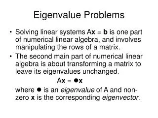
Eigenvalue Problems. Solving linear systems A x = b is one part of numerical linear algebra, and involves manipulating the rows of a matrix. The second main part of numerical linear algebra is about transforming a matrix to leave its eigenvalues unchanged. A x = x

Eigenvalue Problems
E N D
Presentation Transcript
Eigenvalue Problems • Solving linear systems Ax = b is one part of numerical linear algebra, and involves manipulating the rows of a matrix. • The second main part of numerical linear algebra is about transforming a matrix to leave its eigenvalues unchanged. Ax = x where is an eigenvalue of A and non-zero x is the corresponding eigenvector.
What are Eigenvalues? • Eigenvalues are important in physical, biological, and financial problems (and others) that can be represented by ordinary differential equations. • Eigenvalues often represent things like natural frequencies of vibration, energy levels in quantum mechanical systems, stability parameters.
What are Eigenvectors • Mathematically speaking, the eigenvectors of matrix A are those vectors that when multiplied by A are parallel to themselves. • Finding the eigenvalues and eigenvectors is equivalent to transforming the underlying system of equations into a special set of coordinate axes in which the matrix is diagonal. • The eigenvalues are the entries of the diagonal matrix. • The eigenvectors are the new set of coordinate axes.
Determinants • Suppose we if eliminate the components of x from Ax=0 using Gaussian Elimination without pivoting. • We do the kth forward elimination step by subtracting ajk times row k from akk times row j, for j=k,k+1,…n. • Then at the end of forward elimination we have Ux=0, and Unn is the determinant of A, det(A). • For nonzero solutions to Ax=0 we must have det(A) = 0. • Determinants are defined only for square matrices.
Determinant Example • Suppose we have a 33 matrix. • So Ax=0 is the same as: a11x1+a12x2+a13x3 = 0 a21x1+a22x2+a23x3 = 0 a31x1+a32x2+a33x3 = 0
Determinant Example (continued) • Step k=1: • subtract a21 times equation 1 from a11 times equation 2. • subtract a31 times equation 1 from a11 times equation 3. • So we have: (a11a22-a21a12)x2+(a11a23-a21a13)x3 = 0 (a11a32-a31a12)x2+(a11a33-a31a13)x3 = 0
Determinant Example (continued) • Step k=2: • subtract (a11a32-a31a12) times equation 2 from (a11a22-a21a12) times equation 3. • So we have: [(a11a22-a21a12)(a11a33-a31a13)- (a11a32-a31a12)(a11a23-a21a13)]x3 = 0 which becomes: [a11(a22a33 –a23a32) – a12(a21a33-a23a31) + a13(a21a32-a22a31)]x3 = 0 and so: det(A) = a11(a22a33 –a23a32) – a12(a21a33-a23a31) + a13(a21a32-a22a31)
Definitions • Minor Mij of matrix A is the determinant of the matrix obtained by removing row i and column j from A. • Cofactor Cij = (-1)i+jMij • If A is a 11 matrix then det(A)=a11. • In general, where i can be any value i=1,…n.
A Few Important Properties • det(AB) = det(A)det(B) • If T is a triangular matrix, det(T) = t11t22…tnn • det(AT) = det(A) • If A is singular then det(A)=0. • If A is invertible then det(A)0. • If the pivots from Gaussian Elimination are d1, d2,…,dn then det(A) = d1d2dn where the plus or minus sign depends on whether the number of row exchanges is even or odd.
Characteristic Equation • Ax = x can be written as (A-I)x = 0 which holds for x0, so (A- I) is singular and det(A-I) = 0 • This is called the characteristic polynomial. If A is nn the polynomial is of degree n and so A has n eigenvalues, counting multiplicities.
Example • Hence the two eigenvalues are 1 and 5.
Example (continued) • Once we have the eigenvalues, the eigenvectors can be obtained by substituting back into (A-I)x = 0. • This gives eigenvectors (1 -1)T and (1 1/3)T • Note that we can scale the eigenvectors any way we want. • Determinant are not used for finding the eigenvalues of large matrices.
Positive Definite Matrices • A complex matrix A is positive definite if for every nonzero complex vector x the quadratic form xHAx is real and: xHAx > 0 where xH denotes the conjugate transpose of x (i.e., change the sign of the imaginary part of each component of x and then transpose).
Eigenvalues of Positive Definite Matrices • If A is positive definite and and x are an eigenvalue/eigenvector pair, then: Ax = x xHAx = xHx • Since xHAx and xHx are both real and positive it follows that is real and positive.
Properties of Positive Definite Matrices • If A is a positive definite matrix then: • A is nonsingular. • The inverse of A is positive definite. • Gaussian elimination can be performed on A without pivoting. • The eigenvalues of A are positive.
Hermitian Matrices • A square matrix for which A = AH is said to be an Hermitian matrix. • If A is real and Hermitian it is said to be symmetric, and A = AT. • Every Hermitian matrix is positive definite. • Every eigenvalue of an Hermitian matrix is real. • Different eigenvectors of an Hermitian matrix are orthogonal to each other, i.e., their scalar product is zero.
Eigen Decomposition • Let 1,2,…,n be the eigenvalues of the nn matrix A and x1,x2,…,xn the corresponding eigenvectors. • Let be the diagonal matrix with 1,2,…,n on the main diagonal. • Let X be the nn matrix whose jth column is xj. • Then AX = X, and so we have the eigen decomposition of A: A = XX-1 • This requires X to be invertible, thus the eigenvectors of A must be linearly independent.
Powers of Matrices • If A = XX-1 then: A2 = (XX-1)(XX-1) = X(X-1X)X-1 = X2X-1 Hence we have: Ap = XpX-1 • Thus, Ap has the same eigenvectors as A, and its eigenvalues are 1p,2p,…,np. • We can use these results as the basis of an iterative algorithm for finding the eigenvalues of a matrix.
The Power Method • Label the eigenvalues in order of decreasing absolute value so |1|>|2|>… |n|. • Consider the iteration formula: yk+1 = Ayk where we start with some initial y0, so that: yk = Aky0 • Then yk converges to the eigenvector x1 corresponding the eigenvalue 1.
Proof • We know that Ak = XkX-1, so: yk = Aky0 = XkX-1y0 • Now we have: • The terms on the diagonal get smaller in absolute value as k increases, since 1 is the dominant eigenvalue.
Proof (continued) • So we have • Since 1k c1 x1 is just a constant times x1 then we have the required result.
Example • Let A = [2 -12; 1 -5] and y0=[1 1]’ • y1 = -4[2.50 1.00]’ • y2 = 10[2.80 1.00]’ • y3 = -22[2.91 1.00]’ • y4 = 46[2.96 1.00]’ • y5 = -94[2.98 1.00]’ • y6 = -190[2.99 1.00]’ • The iteration is converging on a scalar multiple of [3 1]’, which is the correct dominant eigenvector.
Rayleigh Quotient • Note that once we have the eigenvector, the corresponding eigenvalue can be obtained from the Rayleigh quotient: dot(Ax,x)/dot(x,x) where dot(a,b) is the scalar product of vectors a and b defined by: dot(a,b) = a1b1+a2b2+…+anbn • So for our example, 1 = -2.
Scaling • The 1k can cause problems as it may become very large as the iteration progresses. • To avoid this problem we scale the iteration formula: yk+1 = A(yk /k+1) where k+1 is the component of Ayk with largest absolute value.
Example with Scaling • Let A = [2 -12; 1 -5] and y0=[1 1]’ • Ay0 = [-10 -4]’ so 1=-10 and y1=[1.00 0.40]’. • Ay1 = [-2.8 -1.0]’ so 2=-2.8 and y2=[1.0 0.3571]’. • Ay2 = [-2.2857 -0.7857]’ so 3=-2.2857 and y3=[1.0 0.3437]’. • Ay3 = [-2.1250 -0.7187]’ so 4=-2.1250 and y4=[1.0 0.3382]’. • Ay4 = [-2.0588 -0.6912]’ so 5=-2.0588 and y5=[1.0 0.3357]’. • Ay5 = [-2.0286 -0.6786]’ so 6=-2.0286 and y6=[1.0 0.3345]’. • is converging to the correct eigenvector -2.
Scaling Factor • At step k+1, the scaling factor k+1 is the component with largest absolute value is Ayk. • When k is sufficiently large Ayk 1yk. • The component with largest absolute value in 1yk is 1 (since yk was scaled in the previous step to have largest component 1). • Hence, k+1 1 as k .
MATLAB Code function [lambda,y]=powerMethod(A,y,n) for (i=1:n) y = A*y; [c j] = max(abs(y)); lambda = y(j); y = y/lambda; end
Convergence • The Power Method relies on us being able to ignore terms of the form (j/1)k when k is large enough. • Thus, the convergence of the Power Method depends on |2|/|1|. • If |2|/|1|=1 the method will not converge. • If |2|/|1| is close to 1 the method will converge slowly.
Orthonormal Vectors • A set S of nonzero vectors are orthonormal if, for every x and y in S, we have dot(x,y)=0 (orthogonality) and for every x in S we have ||x||2=1 (length is 1).
Similarity Transforms • If T is invertible, then the matrices A and B=T-1AT are said to be similar. • Similar matrices have the same eigenvalues. • If x is the eigenvector of A corresponding to eigenvalue , then the eigenvector B corresponding to eigenvalue is T-1x. Ax=x TBT-1x=x B(T-1x)=(T-1x)
The QR Algorithm • The QR algorithm for finding eigenvalues is based on the QR factorisation that represents a matrix A as: A = QR where Q is a matrix whose columns are orthonormal, and R is an upper triangular matrix. • Note that QHQ = I and Q-1=QH. • Q is termed a unitary matrix.
QR Algorithm without Shifts A0 = A for k=1,2,… QkRk = Ak Ak+1 = RkQk end Since: Ak+1 = RkQk = Qk-1AkQk then Ak and Ak+1 are similar and so have the same eigenvalues. Ak+1 tends to an upper triangular matrix with the same eigenvalues as A. These eigenvalues lie along the main diagonal of Ak+1.
QR Algorithm with Shift Since: Ak+1 = RkQk + sI = Qk-1(Ak – sI)Qk +sI = Qk-1AkQk so once again Ak and Ak+1 are similar and so have the same eigenvalues. A0 = A for k=1,2,… s = Ak(n,n) QkRk = Ak - sI Ak+1 = RkQk + sI end The shift operation subtracts s from each eigenvalue of A, and speeds up convergence.
MATLAB Code for QR Algorithm • Let A be an nn matrix n = size(A,1); I = eye(n,n); s = A(n,n); [Q,R] = qr(A-s*I); A = R*Q+s*I • Use the up arrow key in MATLAB to iterate or put a loop round the last line.
Deflation • The eigenvalue at A(n,n) will converge first. • Then we set s=A(n-1,n-1) and continue the iteration until the eigenvalue at A(n-1,n-1) converges. • Then set s=A(n-2,n-2) and continue the iteration until the eigenvalue at A(n-2,n-2) converges, and so on. • This process is called deflation.
