Download
1 / 29
300 likes | 386 Views
Quasirandomness. Benjamin Doerr. Max-Planck-Institut für Informatik Saarbrücken. =. ¯. ¯. ¯. ¯. 1. 2. +. j. j. j. j. (. (. ). ). j. j. j. j. (. (. j. j. (. j. j. ). ). ). l. l. l. P. P. R. R. R. R. P. P. O. O. P. P. ". ¡. ¡. . . v. v. o. o.

E N D
Quasirandomness Benjamin Doerr Max-Planck-Institut für Informatik Saarbrücken
= ¯ ¯ ¯ ¯ 1 2 + j j j j ( ( ) ) j j j j ( ( j j ( j j ) ) ) l l l P P R R R R P P O O P P " ¡ ¡ \ \ v v o o o g = = ¯ ¯ ¯ ¯ Introduction to Quasirandomness • Pseudorandomness: • Aim: Have something look completely random • Example: Pseudorandom numbers shall look random independent of the particular application. • Quasirandomness: • Aim: Imitate a particular property of a random object. • Example: Low-discrepancy point sets • A random point set P is evenly distributed in [0,1]2: For all axis-parallel rectangles R, • Quasirandom analogue: There are point sets P such that holds for all R • Leads to (Quasi)-Monte-Carlo methods Benjamin Doerr
Why Study Quasirandomness? • Basic research: Is it truely the randomness that makes a random object useful, or something else? • Example numerical integration: Random sample points are good because of their sublinear discrepancy (and ‘not’ because they are random) • Learn from the random object and make it better (custom it to your application) without randomness! • Combine random and quasirandom elements: What is the right dose of randomness? Benjamin Doerr
Outline of the Talk • Part 0: Introduction to Quasirandomness [done] • Quasirandom: Imitate a particular aspect of randomness • Part 1: Quasirandom random walks • also called “Propp machine” or “rotor router model” • Part 2: Quasirandom rumor spreading • the right dose of randomness? Benjamin Doerr
Part 1: Quasirandom Random Walks • Reminder: Random Walk • How to make it quasirandom? • Three results: • Cover times • Discrepancies: Massive parallel walks • Internal diffusion limited aggregation (physics) Benjamin Doerr
Reminder: Random Walks • Rule: Move to a neighbor chosen at random Benjamin Doerr
Quasirandom Random Walks • Simple observation: If the random walk visits a vertex many times, then it leaves it to each neighbor approximately equally often • n visits to a vertex of constant degree d: n/d + O(n1/2) moves to each neighbor. • Quasirandomness: Ensure that neighbors are served evenly! Benjamin Doerr
Quasirandom Random Walks • Rule: Follow the rotor. Rotor updates after each move. Benjamin Doerr
Quasirandom Random Walks • Simple observation: If the random walk visits a vertex many times, then it leaves it to each neighbor approx. equally often • n visits to a vertex of constant degree d: n/d + O(n1/2) moves to each neighbor. • Quasirandomness: Ensure that neighbors are served evenly! • Put a rotor on each vertex, pointing to its neighbors • The quasirandom walk moves in the rotor direction • After each step, the rotor turns and points to the next neighbor (following a given permutation of the neighbors) Benjamin Doerr
Quasirandom Random Walks • Other names • Propp machine (after Jim Propp) • Rotor router model • Deterministic random walk • Some freedom in the design • Initial rotor directions • Order, in which the rotors serve the neighbors • Also: Alternative ways to ensure fairness in serving the neighbors Fortunately: No real difference Benjamin Doerr
Result 1: Cover Times • Cover time: How many step does the (quasi)random walk need to visit all vertices? • Classical result [AKLLR’79]: For all graphs G=(V,E) and all vertices v, the expected time a random walk started in v needs to visit all vertices, is at most 2 |E|(|V|-1). • Quasirandom [D]: For all graphs, starting vertices, initial rotor directions and rotor permutations, the quasirandom walk needs at most 2|E|(|V|-1) steps to visit all vertices. • Note: Same bound, but ‘sure’ instead of ‘expected’. Benjamin Doerr
Result 2: Discrepancies • Model: Many chips do a synchronized (quasi)random walk • Discrepancy: Difference between the number of chips on a vertex at a time in the quasirandom model and the expected number in the random model Benjamin Doerr
Example: Discrepancies on the Line Random Walk (Expectation): 19 2.375 4.75 7.125 9.5 9.5 7.125 9.5 4.75 2.375 Quasirandom: 19 2 5 8 9 9 10 6 5 3 But: You’ll never have more than 2.29 [Cooper, D, Spencer, Tardos] A discrepancy > 1! Difference: -0.375 0.25 0.875 -0.5 -0.5 -1.125 0.5 0.25 0.625 Benjamin Doerr
Result 2: Discrepancies • Model: Many chips do a synchronized (quasi)random walk • Discrepancy: Difference between the number of chips on a vertex at a time in the quasirandom model and the expected number in the random model • Cooper, Spencer [CPC’06]: If the graph is an infinite d-dim. grid, then (under some mild conditions) the discrepancies on all vertices at all times can be bounded by a constant (independent of everything!) • Note: Again, we compare ‘sure’ with expected • Cooper, D, Friedrich, Spencer [SODA’08]: Fails for infinite trees • Open problem: Results for any other graphs Benjamin Doerr
Result 3: Internal Diffusion Limited Aggregation • Model: • Start with an empty 2D grid. • Each round, insert a particle at ‘the center’ and let it do a (quasi)random walk until it finds an empty grid cell, which it then occupies. • What is the shape of the occupied cells after n rounds? • 100, 1600 and 25600 particles in the random walk model: [Moore, Machta] Benjamin Doerr
Result 3: Internal Diffusion Limited Aggregation • Model: • Start with an empty 2D grid. • Each round, insert a particle at ‘the center’ and let it do a (quasi)random walk until it finds an empty grid cell, which it then occupies. • What is the shape of the occupied cells after n rounds? • With random walks: • Proof: outradius – inradius = O(n1/6) [Lawler’95] • Experiment: outradius – inradius ≈ log2(n) [Moore, Machta’00] • With quasirandom walks: • Proof: outradius – inradius = O(n1/4+eps) [Levine, Peres] • Experiment: outradius – inradius < 2 Benjamin Doerr
Summary Quasirandom Walks • Model: • Follow the rotor and rotate it • Simulates: Random walks leave each vertex in each direction roughly equally often • Results: Surprising good simulation (or “better”) • Graph exploration in 2|E|(|V|-1) steps • Many chips: For grids (but not trees), we have the same number of chips on each vertex at all times as expected in the random walk (apart from constant discrepancy) • IDLA: Almost perfect circle. Benjamin Doerr
Part 2: Quasirandom Rumor Spreading • Reminder: Randomized Rumor Spreading • same as in the talk by Thomas Sauerwald • Quasirandom Rumor Spreading • Purely deterministic: Poor • With a little bit of randomness: Great![simpler and better than randomized] • “The right dose of randomness”? Benjamin Doerr
Randomized Rumor Spreading • Model (on a graph G): • Start: One node is informed • Each round, each informed node informs a neighbor chosen uniformly at random • Broadcast time T(G): Number of rounds necessary to inform all nodes (maximum taken over all starting nodes) Round 4: Each informed node informs a random node Round 5: Let‘s hope the remaining two get informed... Round 2: Each informed node informs a random node Round 3: Each informed node informs a random node Round 1: Starting node informs random node Round 0: Starting node is informed Benjamin Doerr
Randomized Rumor Spreading • Model (on a graph G): • Start: One node is informed • Each round, each informed node informs a neighbor chosen uniformly at random • Broadcast time T(G): Number of rounds necessary to inform all nodes (maximum taken over all starting nodes) • Application: • Broadcasting updates in distributed databases • simple • robust • self-organized Benjamin Doerr
Randomized Rumor Spreading • Model (on a graph G): • Start: One node is informed • Each round, each informed node informs a neighbor chosen uniformly at random • Broadcast time T(G): Number of rounds necessary to inform all nodes (maximum taken over all starting nodes) • Results [n: Number of nodes]: • Easy: For all graphs G, T(G) ≥ log(n) • Frieze, Grimmet: T(Kn) = O(log(n)) w.h.p. • Feige, Peleg, Raghavan, Upfal: T({0,1}d) = O(log(n)) w.h.p. • Feige et al.: T(Gn,p) = O(log(n)) w.h.p., p > (1+eps)log(n)/n Benjamin Doerr
Deterministic Rumor Spreading? • As above except: • Each node has a list of its neighbors. • Informed nodes inform their neighbors in the order of this list. • Problem: Might take long... • Here: n-1 rounds . 1 2 3 4 5 6 List: 2 3 4 5 6 3 4 5 6 1 4 5 6 1 2 5 6 1 2 3 6 1 2 3 4 1 2 3 4 5 Benjamin Doerr
Semi-Deterministic Rumor Spreading • As above except: • Each node has a list of its neighbors. • Informed nodes inform their neighbors in the order of this list, but start at a random position in the list Benjamin Doerr
Semi-Deterministic Rumor Spreading • As above except: • Each node has a list of its neighbors. • Informed nodes inform their neighbors in the order of this list, but start at a random position in the list • Results (1): Benjamin Doerr
Semi-Deterministic Rumor Spreading • As above except: • Each node has a list of its neighbors. • Informed nodes inform their neighbors in the order of this list, but start at a random position in the list • Results (1): The log(n) bounds for • complete graphs, • random graphs Gn,p, p > (1+eps) log(n), • hypercubes still hold... Benjamin Doerr
Semi-Deterministic Rumor Spreading • As above except: • Each node has a list of its neighbors. • Informed nodes inform their neighbors in the order of this list, but start at a random position in the list • Results (1): The log(n) bounds for • complete graphs, • random graphs Gn,p, p > (1+eps) log(n), • hypercubes still hold independent from the structure of the lists [D, Friedrich, Sauerwald (SODA’08)] Benjamin Doerr
Semi-Deterministic Rumor Spreading • Results (2): • Random graphs Gn,p, p = (log(n)+log(log(n)))/n: • fully randomized: T(Gn,p) = Θ(log(n)2) w.h.p. • semi-deterministic: T(Gn,p) = Θ(log(n)) w.h.p. • Complete k-regular trees: • fully randomized: T(G) = Θ(k log(n)) w.h.p. • semi-deterministic: T(G) = Θ(k log(n)/log(k)) w.p.1 • Algorithm Engineering Perspective: • need fewer random bits • easy to implement: Any implicitly existing permutation of the neighbors can be used for the lists Benjamin Doerr
The Right Dose of Randomness? • Results indicate that the right dose of randomness can be important! • Alternative to the classical “everything independent at random” • May-be an interesting direction for future research? • Related: • Dependent randomization, e.g., dependent randomized rounding: • Gandhi, Khuller, Partharasathy, Srinivasan (FOCS’01+02) • D. (STACS’06+07) • Randomized search heuristics: Combine random and other techniques, e.g., greedy • Example: Evolutionary algorithms • Mutation: Randomized • Selection: Greedy (survival of the fittest) Benjamin Doerr
Summary • Quasirandomness: • Simulate a particular aspect of a random object • Surprising results: • Quasirandom walks • Quasirandom rumor spreading • For future research: • Good news: Quasirandomness can be analyzed (in spite of ‘nasty’ dependencies) • Many open problems • “What is the right dose of randomness?” Thanks! Benjamin Doerr