One Dimensional Flow

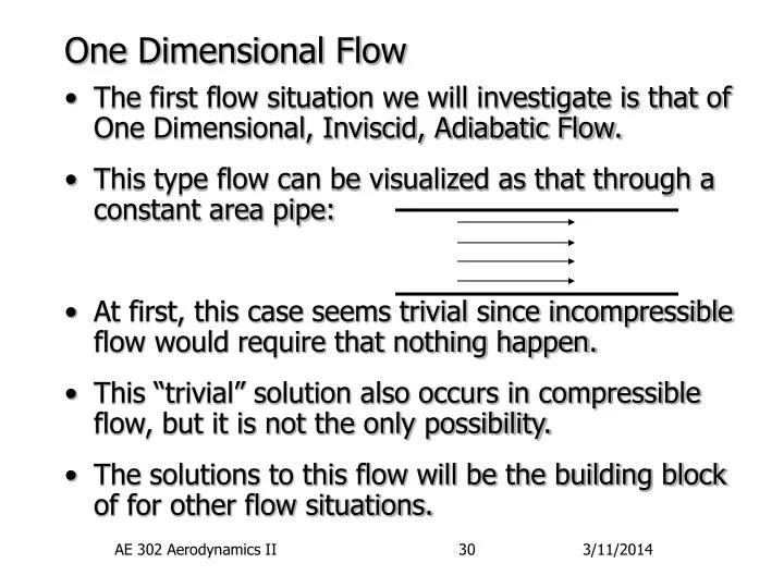
1. One Dimensional Flow • The first flow situation we will investigate is that of One Dimensional, Inviscid, Adiabatic Flow. • This type flow can be visualized as that through a constant area pipe: • At first, this case seems trivial since incompressible flow would require that nothing happen. • This “trivial” solution also occurs in compressible flow, but it is not the only possibility. • The solutions to this flow will be the building block of for other flow situations. AE 302 Aerodynamics II

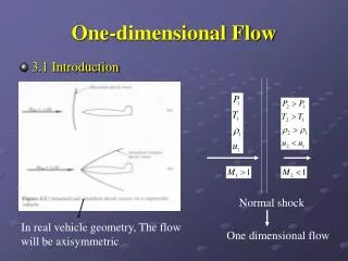
2. Shock wave One Dimensional Flow [2] • There are also a number of ‘nearly’ one dimensional flow situations. • For example the flow in a converging/diverging duct or the flow along the stagnation streamline of a blunt body in supersonic flow: • These are cases of Quasi-One Dimensional Flow which will be discussed in later chapters. AE 302 Aerodynamics II

3. 1-D Flow Equations • For 1-D flow, the velocity reduces to a single component, u, which we will align with the x axis. • We will only consider steady flow, so the mass and momentum conservation equations become: Flow ‘wave’ AE 302 Aerodynamics II

4. 1-D Flow Equations [2] • For the flow through the control volume shown, we allow for the possibility of a flow disturbance in the form of a wave – either a pressure or shock-wave. • By integrating over the inflow/outflow boundaries: Flow ‘wave’ AE 302 Aerodynamics II

5. 1-D Flow Equations [3] • And for the energy equation: • But, from the mass conservation (continuity) equation, 1u1 = 2u2. Thus: AE 302 Aerodynamics II

6. 1-D Flow Equations [3] • If the inflow conditions are known, that leaves us 5 unknowns at the outflow: p2, r2, u2, T2 , h2 . • So far we only have 3 equations – so we need two more relations to obtain a solution. • The enthalpy and temperature are, of course, related: • This thermally perfect relation adds one equation – and the perfect gas law give us the needed 5th. AE 302 Aerodynamics II

7. Speed of Sound • A special case of 1-D flow is that of a very weak pressure wave – i.e., a sound wave. • In this case, put the control volume in motion with the wave so that the inflow velocity is the speed of sound, a. • Also allow for the possibility of a change in flow properties across the wave. • Since a sound wave is weak, express these changes as differential quantities. Sound wave AE 302 Aerodynamics II

8. Speed of Sound [2] • In this case, the conservation of mass becomes (after dropping higher order terms): • And momentum becomes: Sound wave AE 302 Aerodynamics II

9. Speed of Sound [3] • Combine the two equations by eliminating da: • This last expressions is a differentiation and to be precise, it should be a partial differentiation with one other property held constant. • Since the flow is adiabatic and inviscid, it is natural to require isentropic (constant entropy) flow. AE 302 Aerodynamics II

10. Speed of Sound [4] • Thus, the speed of sound can be written as: • Also note, that given our previous definition of the compressibility factor, the speed of sound can also be written as: • Thus we see the close relationship between compressibility and the speed of sound. AE 302 Aerodynamics II

11. Speed of Sound [5] • While the previous equations are interesting in understanding flow behavior, they don’t help much in actual calculations. • To obtain a useful equation, apply our isentropic relation: • If the grouping of properties at the two locations can be separated, they must separately equal a constant. Thus: • As it turns out, we don’t really need to know the value of the constant, C. AE 302 Aerodynamics II

12. Speed of Sound [6] • Instead, it can be eliminated when we perform the differentiation: • And thus, • Also, the perfect gas low can be used to obtain: • Note this dependence on temperature, and thus the speed of the random motion of the particles, also makes good sense. AE 302 Aerodynamics II

13. Forms of the Energy Equation • Before going on, it is important to spend a little time considering different forms of the energy eqn. • As before, if the properties at two locations can be separated, they must each equal a constant. • For this case, we will give the constant a name – the total enthalpy. • We indicate this ‘total’ property with a subscript zero since it is also the value at zero velocity. • From incompressible flow, we might also call this the ‘stagnation’ enthalpy. AE 302 Aerodynamics II

14. Forms of the Energy Equation [2] • We can also use the relationship between enthalpy and temperature to write either of: • Further, if the relation between the speed of sound and temperature is introduced… • Then, we get: AE 302 Aerodynamics II

15. Forms of the Energy Equation [3] • All the previous equations are valid forms of the adiabatic energy equation. • One form relates the properties at two points in a flow to each other while the other form relates the properties at any point to the reference, total conditions. • This is useful since, for adiabatic flow, the total flow conditions of ho, To, and aodo not change! • We will later see that these 1-D equations are also valid in 2 and 3-D if the velocity is replaced with the total velocity magnitude: u  V AE 302 Aerodynamics II

16. Forms of the Energy Equation [4] • For external flows, the total or stagnation conditions are the preferred reference values. • In internal flows, like engines, there is another set of reference conditions often used. These are the sonic conditions – or those that would occur at the speed of sound. • Using an asterisk to denote sonic conditions, one form of the energy equation is: • Note that by definition: AE 302 Aerodynamics II

17. Forms of the Energy Equation [5] • Similarly, the sonic temperature can be introduced: • Note also that the sonic and total conditions can be related: • Thus: • If follows that these sonic conditions, like the total conditions are flow constants. AE 302 Aerodynamics II

18. Mach Relation • Some final, and probably the most useful, forms of the energy equation involve the Mach number. • Rearrange to get the ratio of total to local temperature on one side: • Now, introduce the Mach number to get the first of our “Mach Relation” equations: AE 302 Aerodynamics II

19. Limits of Adiabatic Flow Assumption • All of the equations to this point are valid for any adiabatic flow – which is pretty much all aerodynamic flow cases. • However, there are some important situations where the above equation doesn’t work: • Obviously, whenever there is heat addition – the most common of which is actively cooled hypersonic and space reentry flows. • Whenever there is a propeller, compressor, or turbine. • Two merging flows from separate sources. • In these cases, the equations don’t work because the total enthalpy is not a constant – and thus neither is the total temperature. AE 302 Aerodynamics II

20. Limits of Adiabatic Flow Assumption [2] • This brings up an important point – the total (and sonic) conditions are reference conditions, they don’t necessarily correspond to a point in the flow. • However, all points in a flow have a total and sonic temperature associated with them – these are a measure of the energy at the point. • In the cases mentioned, the energy (internal plus kinetic) is not a constant throughout: T01 T02 >T01 T01 T02 AE 302 Aerodynamics II

21. Isentropic Flow Relations • While the previous equations are good for any adiabatic flow, there are also many cases when the flow is also reversible – and thus isentropic. • From our previous isentropic flow relations: • These equations relate the properties at one locations to that of another – as long as the flow between the two points is isentropic! • Thus, this equation will not work in a viscous boundary layer or across a shock wave. AE 302 Aerodynamics II

22. Isentropic Flow Relations [2] • We can use these equations to also calculate the total pressure and total density: • As with the total enthalpy and temperature, these reference quantities don’t have to be actual points in the flow. • Thus, the total pressure is the pressure the flow would have IF it were isentropic brought to rest. • Similarly, the total density is the density the flow would have IF isentropically brought to rest. AE 302 Aerodynamics II

23. Isentropic Flow Relations [3] • Using these relations, we can then write: • And the sonic pressure and temperature can be found from: AE 302 Aerodynamics II

24. Dynamic Pressure • When non-dimensionalizing forces and pressures in compressible flow, it is still convenient to use the dynamic pressure. I.e.: • However, remember that Bernoulli’s equation does not apply in compressible flow! • To reinforce this, we can rewrite the dynamic pressure in terms of pressure and Mach number: AE 302 Aerodynamics II

25. Normal Shock Relations • Finally, let’s return to our original problem and look at the case when a shock wave is present. • In particular, this is called a normal shock because it is perpendicular to the flow. • The conservations equations in 1-D are still: Shock Wave AE 302 Aerodynamics II

26. Normal Shock Relations [2] • Let’s start by dividing the two sides of the momentum by the mass conservation equation: • And, by rearranging and introducing the speed of sound: • But, from one form of our energy equation: AE 302 Aerodynamics II

27. Normal Shock Relations [3] • Or, when written for the two points involved: • Note that since the flow is adiabatic, the sonic speed of sound, a*, is the same at both points. • Substituting these two equations into our previous equation – and rearranging – gives: • Which looks complex - until you notice the common factor (u2-u1). AE 302 Aerodynamics II

28. Normal Shock Relations [4] • This equation is automatically satisfied if nothing happens in the control volume, i.e. u2=u1. • This is the trivial case, but it is nice to know our equations will give that result. • The more interesting case is when (u2-u1) 0, which allows us to divide through by this factor. • Or, when rearranged, simply: AE 302 Aerodynamics II

29. Characteristic Mach Number • Another way of writing this result is in terms of the characteristic Mach number: M* = u/a*. • Note that this is not a “true” Mach number which is the ratio of local velocity to local speed of sound. • This relationship tells us something very important • If the flow is initially subsonic, u1<a*, then it will become supersonic u2>a*. • Of, if the flow is initially supersonic, u1>a*, then it will become subsonic, u2<a*. AE 302 Aerodynamics II

30. Characteristic Mach Number [2] • The first possibility, a flow spontaneously jumping from subsonic to supersonic, isn’t physically possible - we will show this in a little bit. • The second case, jumping from supersonic to subsonic is exactly what a normal shock does. • Why? Usually because there is some disturbance or condition downstream which the flow cannot negotiate supersonically. I.e: • When there is a blunt body the flow must go around • When a nozzle has an exit pressure condition which requires subsonic flow AE 302 Aerodynamics II

31. Characteristic Mach Number [3] • The previous characteristic Mach relation, while informative, is not very useful in application. • Instead, relate the characteristic Mach to the true Mach number by using: • When simplified, this becomes: • Thus the two values are (relatively) simply related. AE 302 Aerodynamics II

32. Mach Jump Relation • Substituting into our characteristic Mach relation: • Or, when simplified, we get the useful relation: AE 302 Aerodynamics II

33. Mach Jump Relation [2] • It is important to note the limits of the expression as M11 and M1. • Thus, if we are sonic, the normal shock becomes very week and nothing happens. • If we go hyper-hypersonic, the flow reaches a fixed post-shock Mach number. AE 302 Aerodynamics II

34. Density/Velocity Jump Relation • To get the shock jump relations for our remaining flow properties, start with continuity: • Thus, the density and velocity jumps are inversely related and given by: AE 302 Aerodynamics II

35. Density/Velocity Jump Relation [2] • Once again, if M1=1, the shock wave becomes very weak and nothing happens. • At very high speeds, however: • Thus, when you hear some people talk about hypersonic vehicles compressing air to the density of steel…. • Well, not quite. Not even close actually. But it sure sounds impressive. AE 302 Aerodynamics II

36. Pressure Jump Relation • Next, turn to momentum conservation to get a relation for pressure. First rearrange terms: • And them manipulate to get Mach numbers and our previous velocity jump expression: • Or, just AE 302 Aerodynamics II

37. Pressure Jump Relation [2] • Finally, insert our definition for characteristic Mach number…. • And, on simplification: AE 302 Aerodynamics II

38. Pressure Jump Relation [3] • Once again if M1=1, nothing happens. • Note that this time however, as M1, the pressure also does: • Thus, while the density might not be huge, the pressures can be. • Finally, the easiest way to get the temperature jump is through the perfect gas law: • So, temperatures also get very large! AE 302 Aerodynamics II

39. Entropy Change • And last, consider the change in entropy across a normal shock wave. • Using our previous definition and the perfect gas law: • Or with a little extra manipulation: AE 302 Aerodynamics II

40. Entropy Change [2] • Now, insert our shock jump relations: • Now we see that a subsonic shock, M1<1 would produce a decrease in entropy – something not allowed by the 2nd Law of Thermodynamics. • Thus only supersonic shocks are possible. AE 302 Aerodynamics II

41. Total Pressure Jump • One final thing to note is this special case where a flow is: • isentropically accelerated from rest to M1 • jumps through a shock • and then isentropically slows back down to rest. • The only entropy change occurs at the shock, thus, we can write for the initial and final states: • Or, since the flow is adiabatic, T01 = T02. Thus: AE 302 Aerodynamics II

42. Total Pressure Jump [2] • This can be rewritten as: • As a result, flow efficiency in inlets and nozzles is often measured by this total pressure ratio. • Thus we see the close relationship between entropy changes and total pressure loss. AE 302 Aerodynamics II