Download
1 / 66
800 likes | 1.33k Views
8. The Group SU(2) and more about SO(3). SU(2) = Group of 2 2 unitary matrices with unit determinant. Simplest non-Abelian Lie group. Locally equivalent to SO(3); share same Lie algebra. Compact & simply connected All IRs are single-valued.

E N D
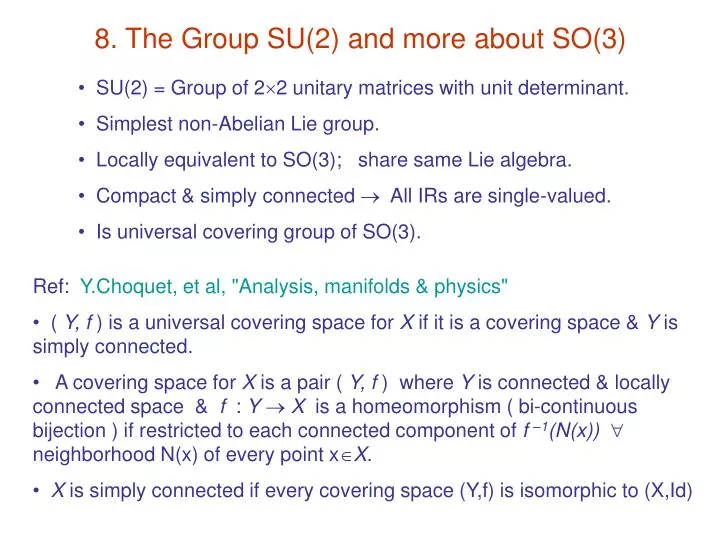
8. The Group SU(2) and more about SO(3) • SU(2) = Group of 22 unitary matrices with unit determinant. • Simplest non-Abelian Lie group. • Locally equivalent to SO(3); share same Lie algebra. • Compact & simply connected All IRs are single-valued. • Is universal covering group of SO(3). • Ref: Y.Choquet, et al, "Analysis, manifolds & physics" • ( Y, f ) is a universal covering space for X if it is a covering space & Y is simply connected. • A covering space for X is a pair ( Y, f ) where Y is connected & locally connected space & f : Y X is a homeomorphism ( bi-continuous bijection ) if restricted to each connected component of f –1(N(x)) neighborhood N(x) of every point xX. • X is simply connected if every covering space (Y,f) is isomorphic to (X,Id)
8.1 The Relationship between SO(3) and SU(2) 8.2 Invariant Integration 8.3 Orthonormality and Completeness Relations of 8.4 Projection Operators and Their Physical Applications 8.5 Differential Equations Satisfied by the D j – Functions 8.6 Group Theoretical Interpretation of Spherical Harmonics 8.7 Multipole Radiation of the Electromagnetic Field U(n): Number of real components = 2 n2 Number of real constraints = n + 2 (n2–n)/2 = n2 Dimension = n2 Dimension of SU(n) = n2 –1
8.1. The Relationship between SO(3) and SU(2) Proved in §7.3: Converse is also true. Proof ( of Theorem 8.1): Let Unitarity condition: i.e. Ansatz:
must hold , n, m = integers ( m = 0 only ) There's no loss of generality in setting n = 0. or Ansatz: Theroem 8.1: U(2) matrices: 4-parameters
Corollary: SU(2) matrices: 3-parameters However, this range of & covers twice the area covered by & . One compromise, chosen by Tung, is to set 0 < < 2. SU(2) matrices form a double-valued rep of SO(3)
Cartesian parametrization of SU(2) matrices: with Group manifold = 4–D spherical surface of radius 1. Compact & simply-connected.
SU(2) SO(3) Let & where i are the Pauli matrices Let Since X is hermitian & traceless, so is X'. i.e., Mapping with is 2-to-1 ( A to same R )
Let ( r1, r2, r3 ) be the independent parameters in the Cartesian parametrization. i.e. & Near E, we have k = 1,2,3 i.e., { k } is a basis of the Lie algebra su(2). Since su(2) & so(3) are the same if we set Since SU(2) is simply-connected, all IRs of su(2) are also single-valued IRs of SU(2)
Higher dim rep's can be generated using tensor techniques of Chap 5: • IRs are generated by irred tensors belonging to symm classes of Sn. • Totally symmetric tensors of rank n form an (n+1)-D space for the j = n/2 IR of SU(2) [ See Example 2, §5.5 ] • Explicit construction of Let where Spinor: Under rotation: i.e. Totally symmetric tensor in tensor space V2n: ( n+1 possible values )
n+1 independent 's in (convenient) normalized form: { [m] } transforms as the canonical components of the j = n/2 IR of su(2): c.f. Problem 8.5 Derivation: see Hamermesh, p.353-4 Correctness of Eq(8.1-25)
8.2. Invariant Integration Also holds for different parametrizations of same group element Specific method for SU(2) to find : Let A, A', & B be prarametrized by resp. e.g., with { ri } { r'i } is orthogonal ( r r' is linear )
Since where where Integrate over r0
Switching to { , , } parametrization Integrate over r
Theorem 8.2: Invariant Integration Measure Let A() be a parametrization of a compact Lie group G & define by where { J } are the generators of the Lie algebra g. Then with Proof: Let A() be another parametrization. Consider any point under different parametrizations. We have ( as required )
Let { i } be the local coordinates at A. For a fixed element B, the coordinates at BA is i.e., In case another parametrization { i } is used at BA, we have QED
Another choice of generators { J' } can always be expressed as a linear combination of the old generators { J } , i.e., where S is independent of coordinates. Example: SU(2) with Euler angle parametrization ( , , )
Example: SU(2) with Euler angle parametrization ( , , ) With the help ofMathematica, we get
C is an arbitrary constant Normalized invariant measure: Group volume
Rearrangement lemma for SU(2): ( Left invariant ) Left & right invariant measures coincide for compact groups. See Gilmore or Miller for proof.
8.3. Orthonormality and Completeness Relations of D j • The existence of an invariant measure, • which is true for every compact Lie group, • establishes the validity of the rearrangement theorem, • which in turn guarantees that • Every IR is finite-dimensional. • Every IR is equivalent to some unitary representation. • A reducible representation is decomposable. • The set of all inequivalent IRs are orthogonal & complete.
Theorem 8.3: Orthonormality of IRs for SU(2) • dA is normalized • nj = 2j+1 In the Euler angle parametrization scheme [ dj() = real ]: ( no sum over n, m )
Theorem 8.4: Completeness of D[R] (Peter-Weyl) The IR D (A)mn form a complete basis in L2(G). L2(G) = ( Hilbert ) space of (Lebesgue) square integrable functions defined on the group manifold of a compact Lie group G. i.e., For G = SU(2),
( completeness ) • Comment: • C.f. Fourier theorem in functional analysis. • f(A) can be vector- or operator- valued.
Bosons Fermions : Bosons Fermions : i.e. both cases
Often, with = n, or, n+ ½ For = 0 Setting (,) → (,) gives i.e., the spherical harmonics { Ylm } forms an orthonormal basis for square integrable functions on the unit sphere. Peter-Weyl:
8.4. Projection Operators & their Physical Applications Transfer operator: c.f. Chap 4 if non-vanishing, transforms like the IBVs { | j m } under SU(2) / SO(3) i.e., (error in eq8.4-2) Henceforth, indices within | or | are exempted from summation rules
8.4.1. Single Particle State with Spin Intrinsic spin = s states of particle in rest frame are eigenstates of J2 with eigenvalue s(s+1) . Denote these states by with Task: Find | p 0, i.e., find X
Alternatively, treating J & P as the generators of rotation & translation, resp, (eq 9.6-5) ( Theorem 9.12 ) Similarly, Prove it ! J·P , P , J2, J3share the same eigenstates Let be the "standard state" . Then L3 = 0 since motion is along z ( Helicity = )
Let where and ( Problem 8.1 ) i.e., helicity of a particle is the same in all inertial frames.
States with definite angular momentum (J, M) : | & | excluded from summation c.f. Peter-Weyl Thm, eq(8.3-4)
For a spinless particle, s = = 0: c.f. § 7.5.2 where
{ | p J M ; fixed } is complete for 1-particle states can be inverted using to give Standard state : D diagonal Traditional description: eigenstates of P2, L2, L3, S3 : with Difficulty: L3, S3 not conserved Helicity is preferred Partial remedy:
8.4.2. Two Particle States with Spin Group theoretical methods essential to avoid complications such as the L–S & j–j coupling schemes. Standard state: C.M. frame, , ,
{ | p J M 1, 2 ; j fixed } is complete for 2-particle states See Jacob & Wick, Annals of Physics (NY) 7, 401 (59) • Advantages of the helicity states: • All quantum numbers are measurables. • Relation between linear- & angular- momentum states is direct: there is no need for the coupling-schemes. • Well-behaved under discrete symmetries. • Applicable to zero-mass particles. • Simplifies application to scattering & decay processes.
8.4.3. Partial Wave Expansion for 2-Particle Scattering with Spin Initial state: Final state: • All known interactions are invariant under SO(3). • Scattering matrix preserves J. Wigner–Eckart theorem:
( General partial wave expansion for 2-particle scattering ) c.f. §§ 7.5.3, 11.4, 12.7 Static spin version would involve multiple C–GCs.
8.5. Differential Equations Satisfied by the D j– Functions 1-D translation (§6.6): Functions { e– i x p } are IRs of Lie group T1.
Tung's version is described in SU(2).ppt & R.nb The following derivations are Mathematica assisted. See R_New.nb
Using
(1) (2) (3) (3) + i sin (2) – cos (1) : (3) – i sin (2) – cos (1) :
( Differential equation for D j )
The J eqs give the recurrence relations The J3 equation is the identity: Since the J's are independent of ,, & , we have Note reversed order
For m = 0, j must be an integer & D j is independent of . Let ( j, m') = ( l, m ) & ( ,) = (,), we have
d j is related to the Jacobi polynomials by [ Eq(8.5-13) is wrong ]: From (MathematicaR_New.nb) we have In particular, setting ( j,n,m ) ( l,m,0 ) gives For n = m = 0:
8.6. Group Theoretical Interpretation of Spherical Harmonics Special functions ~ Group representation functions • Roles played by Ylm(,) : • They are matrix elements of the IRs of SO(3). • They are transformation coefficients between bases | & | l m .