Download
1 / 6
60 likes | 175 Views
Comparison of ECMWF Weather Model Precipitation to TRMM Christopher Kidd, NASA GSFC / Code 612 and UMD/ ESSIC. a).

E N D
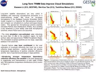
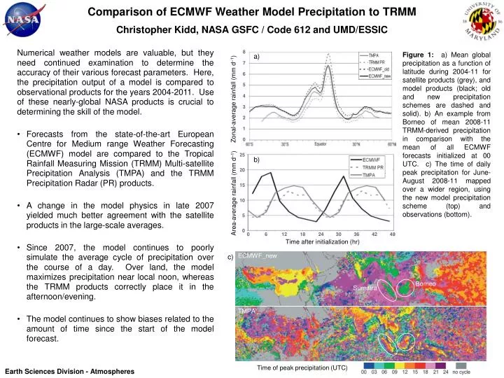
Comparison of ECMWF Weather Model Precipitation to TRMMChristopher Kidd, NASA GSFC/ Code 612 and UMD/ESSIC a) • Numerical weather models are valuable, but they need continued examination to determine the accuracy of their various forecast parameters. Here, the precipitation output of a model is compared to observational products for the years 2004-2011. Use of these nearly-global NASA products is crucial to determining the skill of the model. • Forecasts from the state-of-the-art European Centre for Medium range Weather Forecasting (ECMWF) model are compared to the Tropical Rainfall Measuring Mission (TRMM) Multi-satellite Precipitation Analysis (TMPA) and the TRMM Precipitation Radar (PR) products. • A change in the model physics in late 2007 yielded much better agreement with the satellite products in the large-scale averages. • Since 2007, the model continues to poorly simulate the average cycle of precipitation over the course of a day. Over land, the model maximizes precipitation near local noon, whereas the TRMM products correctly place it in the afternoon/evening. • The model continues to show biases related to the amount of time since the start of the model forecast. 8 Figure 1:a) Mean global precipitation as a function of latitude during 2004-11 for satellite products (grey), and model products (black; old and new precipitation schemes are dashed and solid). b) An example from Borneo of mean 2008-11 TRMM-derived precipitation in comparison with the mean of all ECMWF forecasts initialized at 00 UTC.c) The time of daily peak precipitation for June-August 2008-11 mapped over a wider region, using the new model precipitation scheme (top) and observations (bottom). 7 6 5 4 Zonal-average rainfall (mm d–1) 3 2 1 0 ECMWF_new c) 25 b) Borneo Sumatra 20 15 TMPA Area-average rainfall (mm d–1) 10 5 0 Time of peak precipitation (UTC) 0 6 12 18 24 30 36 42 48 Earth Sciences Division - Atmospheres Time after initialization (hr)
Name: Christopher Kidd, NASA/GSFC/612 and UMD/ESSIC E-mail: chris.kidd@nasa.gov Phone: 301-614-6091 References: Kidd, C., E. Dawkins, G.J. Huffman, 2013: Comparison of Precipitation Derived from the ECMWF Operational Forecast Model and Satellite Precipitation Data Sets. Journal of Hydrometeorology, 14(5), doi:10.1175/JHM-D-12-0182.1, 1463-1482. Contributor: George J. Huffman (NASA/GSFC/612). Data Sources: TRMM Multi-Satellite Precipitation Analysis (TMPA, product 3B42), TRMM Precipitation Radar (product 2A25), European Centre for Medium range Weather Forecasting (ECMWF) operational forecasts. Technical Description of Figures: Figure 1: a) The zonal-average latitudinal profile of precipitation for the TMPA (calibrated to the TRMM combined radiometer-radar product) exceeds that of the PR, but both the “old” and “new” ECMWF forecast model results exceed the TMPA, except for the new ECMWF in the Equatorial and northern Tropics, so the TRMM product difference is not a serious issue. b)The mean (2008-2011) two-day forecast initialized at 0 UTC for Borneo shows that the model peaks much too early and sharply, synchronized with the solar insolation. There is also a spin-up/spin-down problem, in which the first day is systematically different from the second day, even though these long-term averages for the two should be identical. c) The time of the daily peakprecipitation for June-August 2008-11 shows that the model peak-precipitation times are too constant, typified by near-coastal areas in Borneo and Sumatra (circled). These issues are endemic to numerical models; it is important to realize that this is true even for the state-of-the-art ECMWF. Scientific significance: Satellite-based retrievals of precipitation provide a global perspective that is not available from surface-based observations. As such, satellite precipitation data sets can directly address the many scientific and societal benefit areas that require precipitation data, including: the global water and energy cycles; the state and direction of the global climate; storm structures and large-scale atmospheric processes; precipitation microphysical processes; disaster analysis and relief; analysis and forecasting for water resources, agriculture, drought, streamflow and floods, and landslides; risk assessment for civil engineering and insurance; and validating weather and climate forecast models. For the last topic, this paper provides a careful analysis of a particular state-of-the-art numerical weather forecast model, the ECMWF, over a generous multi-year period. The deficiencies shown are typical of such models, including excessive precipitation in the tropical region, inability to correctly depict the diurnal cycle of precipitation, and the “spin-up/spin-down” artifacts early in the model forecast run. The ECMWF implemented a new convective parameterization in November 2007, and this study shows that the change was successful at reducing the overall tropical precipitation bias, but it failed to substantially address the diurnal-cycle problem. It is a matter for future research for other models to address the high bias in the tropics, as the ECMWF has started to do, and for models in general to achieve more-accurate depictions of the diurnal cycle. Many of the areas listed above, particularly streamflow, floods, landslides, and risk assessment, are sensitive to these issues. In contrast to this analysis at lower latitudes, it is likely that the TMPA is somewhat low at higher latitudes, so the higher values for the ECMWF at higher latitudes are considered plausible. However, the diurnal cycle issue remains a problem at higher latitudes. Relevance for Future Missions: The low bias of the satellite retrievals at higher latitudes is a known problem that is being addressed in the Global Precipitation Measurement mission, in studies using CloudSat data, and in related Precipitation Measurement Missions work. The light rain and snow that typify precipitation at higher latitudes require new approaches to retrieval algorithms and, potentially, better channel selections in future satellite sensors. Continued development of numerical model microphysical representations requires improved observational datasets with parameters that more effectively constrain the model’s behavior. This requires new suites of sensors beyond GPM to better retrieve ice crystal populations and vertical velocities, flying on low-orbit satellites that provide near-global coverage. Close interactions between modelers and precipitation scientists is key to the best outcome. Earth Sciences Division - Atmospheres
An Innovative Approach to Separate Thin Cirrus from Aerosols Using High Resolution Ground Spectra R.A. Hansell (UMD-ESSIC/613), S.-C. Tsay (613), P. Pantina (SSAI/613), J. R. Lewis. Q. Ji., J.R. Herman For years, the principles of derivative spectroscopy have been widely used in the field of analytical chemistry for fingerprinting the composition of materials. Hansell et al. 2014 apply these techniques using hyperspectral remote sensing data (http://smartlabs.gsfc.nasa.gov/) from BASE-ASIA 2006 (Tsay et al. 2013), to help discern subtle changes in the spectral signatures of aerosols and cirrus clouds. Differences in spectral slopes are highly dependent on the refractive indices of the medium as well as particle size (Fig. 1). Moreover, the aerosol’s affinity for water, which change both the size and composition of particles, can also affect the shape of the spectrum. An algorithm employing a two-model fit of derivative spectra was developed to determine the relative contributions of aerosols/clouds to measured solar spectra from a ground-based spectroradiometer. When aerosols/cirrus (particularly thin cirrus) coexist, (frequently observed during BASE-ASIA), the cloud optical thickness can be separated from retrieved aerosol optical thickness measurements. The peaks (Fig. 2) coincide with maximum changes in spectral flux, while the magnitude and phase differences in the derivatives are related to the physical and chemical properties in the media. Applications of this approach using hyperspectral, remote-sensing data can provide valuable insight into the aerosol and cloud properties of Earth’s atmosphere. Fig. 1. Observed (o) /modeled (m) spectra of thin cirrus clouds (blue) and heavy biomass burning smoke aerosols (red) during BASE-ASIA. For reference, a clear-sky reference (green) is shown. Depicted slopes (cyan/black curves) illustrate the unique spectral features in the media. Fig. 2. Example derivative spectrum of spectral flux measurements (obs. - black) and aerosol(red)/cirrus (blue) models. Shown are second order derivatives from λ=375-500nm, in the range where variability in the measurements is largest. Earth Sciences Division - Atmospheres
Name: Richard A. Hansell Jr. Email: Richard.A.Hansell@nasa.gov Phone:301.614.6132 • References: • Hansell, R.A., S.-C. Tsay, P. Pantina, J. R. Lewis. Q. Ji., J.R. Herman, 2013: Spectral Derivative Analysis of Solar Spectroradiometric Measurements: Theoretical Basis, J. Geophys. Res. [submitted] • Tsay, S., N.C. Hsu, W.K.-M. Lau, C. Li, P.M. Gabriel, Q. Ji, B.N. Holben, E.J. Welton, A.X Nguyen, S. Janjai, N-H. Lin, J.S. Reid, J. Boonjawat, S.G. Howell, B.J. Huebert, J.S. Fu, R.A. Hansell, A.M. Sayer, R. Gautam, S-H. Wang, C.S. Goodloe, L.R. Miko, P.K. Shu, A.M. Loftus, J. Huang, J.Y. Kim, M.-J. Jeong, and P. Pantina (2013). From BASE-ASIA toward 7-SEAS: A satellite-surface perspective of boreal spring biomass-burning aerosols and clouds in Southeast Asia Atmos. Env, 78, 20-34 doi:10.1016/j.atmosenv.2012.12.013 • Tsai, F., and W. Philpot 1998, Derivative analysis of hyperspectral data, Remote Sens. Environ., 66:41–51. • Carr, S.B., 2005: The aerosol models in MODTRAN: incorporating selected measurements from northern Australia. Technical report DSTO-TR-1803, Defence Science and Technology Organisation, Edinburgh, South Australia, Australia. • Data Sources: NASA SMARTLabs measurements (http://smartlabs.gsfc.nasa.gov); • Technical Description of Figures: • Figure 1: Model (dashed line) versus observed (solid line) spectra for optically thin cirrus (blue curves) and aerosol (red curves) for two ‘near extreme’ cases identified by MPLNET and AERONET data during the 2006 BASE-ASIA field campaign. Also shown for reference is a clear-sky spectrum (green). The two cases are defined by (1) low aerosol loading (AOT ~0.16) under high-level cirrus conditions and (2) high aerosol loading (AOT ~1.1) with no detectable cirrus. The former case was calculated as a mixed cirrus-aerosol scene using the MODTRAN (v.5.2.0.0) radiative transfer code. Aerosols are based on a biomass burning smoke model developed by Carr et al. (2005), while thin ice clouds are defined by MODTRAN’s 4μm mode radius sub-visual cirrus model. Clearly, cirrus and smoke aerosols (both measurements and model) exhibit opposite slopes across the spectral range λ=500-700nm, where the cirrus/smoke slopes are negative/positive, respectively. The slopes are of opposite sign because the absorption coefficients in the media increase/decrease over this bandwidth. • As shown, the cirrus model compares favorably with the measurements having near identical slopes (cyan lines), while that for aerosol (black lines), although reasonable, exhibits a slightly steeper slope than the measurements. This is attributed to the much larger compositional parameter space of aerosols over ice. These cases clearly demonstrate the utility of employing a derivatives-based approach for partitioning atmospheric media. • Figure 2: Smoothed second order derivative spectrum from λ=375-500nm for observed and modeled data (aerosols/cirrus). Positive peaks, identified by their associated downward zero-crossings, correspond to the wavelengths employed in the fitting algorithm used to separate COT from retrieved AOT measurements. Note that features in the modeled aerosol spectrum (red curve) closely follow with those found in the measurements (black curve). Differences in the peak positions and magnitudes coincide with the media’s physical and chemical properties. • Scientific significance: This study illustrates the significance of employing spectral derivatives analysis for studying hyperspectral remote sensing data of Earth’s atmosphere. This technique allows for subtle spectral features to be enhanced which may not be so apparent in the original spectra. Differences in the spectral slopes and peak positions yield important clues for distinguishing aerosols from clouds. More specifically, this technique has the ability to discern optically thin cirrus, which is a well known problem in aerosol remote sensing. This is a valuable tool that can help reveal more detailed structural features in the spectral data. • Relevance for future science and relationship to Decadal Survey: This method offers ways by which the maximum informational content of high spectral resolution measurements can be extracted for Earth science applications. Benefits include (1) improved atmospheric remote sensing capabilities compared to conventional approaches using multi-channel, narrow band measurements and (2) the ability to resolve details in the fine optical structure of aerosols and clouds which can help complement modeling studies. Although derivatives of up to order two likely contain the signal’s maximum spectral content, further work will explore the efficacy of employing higher order derivatives to examine particle shapes, aerosol mixtures, etc. Earth Sciences Division - Atmospheres
Aura OMI Reveals Solar Variability in the on-Going Cycle 24 Sergey Marchenko and Matthew DeLand SSAI, NASA GSFC/Code 614 • Determining long-term solar variations at wavelengths greater than 300 nm requires very accurate satellite measurements, and is needed to quantify natural forcing of Earth’s climate. • The excellent stability of Aura’s Ozone Monitoring Instrument (OMI) allows us to determine short-term (solar rotation) and long-term (solar cycle) solar irradiance variability between 265-500 nm. The difference between solar maximum (2012-2013) and solar minimum (2007-2009) is shown for Cycle 24. • For the first time, we confirm that the magnitude and spectral dependence of short-term and long-term solar irradiance variations are consistent to within derived uncertainties. Variations in solar absorption features closely follow the well-known Mg II index of solar activity, as expected. These new results from OMI are more accurate than previous observations from UARS SUSIM and SOLSTICE during Cycles 22-23. • OMI short-term solar variations agree with concurrent results from the GOME-2 instrument on the ESA MetOp satellite, and with results observed during previous solar cycles. OMI long-term solar variations agree with calculated changes from the NRLSSI model, but disagree with Cycle 23 results from SORCE SIM and SORCE SOLSTICE. FIGURE 1. The spectral dependence of solar variations as observed by Aura OMI; major spectral identified features include Mg II, denoting an absorption line produced by ionized magnesium, and CH, corresponding to a molecular band. The blue line shows the difference between monthly average spectra from solar maximum (2012-2013) to solar minimum (2007-2009). Red lines are typical 2-σ error bars. The black line indicating short-term variations is the average from 8 solar rotations during 2012-2013. Adapted from Marchenko and DeLand[2014, submitted to Ap. J.]. Earth Sciences Division - Atmospheres
NAME: Sergey Marchenko, SSAI, Code 614 E-MAIL:sergey.marchenko@ssaihq.com PHONE: 301-867-6346 REFERENCE: S. Marchenko and M. T. DeLand, “Sun as a Star with Aura OMI: Spectral Changes in the on-Going Cycle 24”, submitted to The Astrophysical Journal, January 2014. DATA SOURCES: Blue– the scaled long-term solar variability spectrum for solar cycle 24 derived from Aura OMI measurements. Red - representative 2-sigma error bars. Black – the short-term solar variability spectrum for the maximum activity level of Cycle 24 derived from OMI measurements. TECHNICAL DESCRIPTION OF FIGURE: The long-term solar variability spectrum for OMI (blue line) is derived from the ratios of monthly averages of the degradation-corrected irradiance spectra between high solar activity years (2012-2013) and low solar activity years (2007-2009). The same month is chosen for each ratio (e.g. March 2013/March 2009) to avoid residual viewing angle errors in the instrument calibration. Data collected during November-January are excluded for the same reason. The result shown here combines all such monthly ratios. The short-term solar variability spectrum for OMI (black line) is derived from the ratio of selected daily irradiance spectra during high solar activity in 2012-2013. The amplitude of each solar rotation (approximately 27-day period) is determined by calculating the ratio of the spectra around the date of the current rotational maximum to the spectra around adjacent minima (both before and after the maximum). Eight rotational cycles between July 2012 and April 2013 were used for this analysis, and the result shown in Figure 1 combines data from all rotations. The representative 2-sigma error bars at selected wavelengths (red) are provided for both the long-term and short-term variability spectra. SCIENCE SIGNIFICANCE: Our results provide the first direct demonstration that the spectral dependence of long-term and short-term solar irradiance variability is in good agreement. By combining our data with previous results and GOME-2 data, we can also provide a consistent representation of short-term solar variability over the extended spectral range 170-795 nm. These data also indicate that, in order to improve the accuracy of spectral retrievals, the users who assume a constant solar spectrum for analysis of atmospheric trace gases (e.g., SO2, NO2, O3, HCHO, BrO) should consider incorporating solar variations, particularly over timescales of weeks to months. Earth Sciences Division - Atmospheres