Download

1 / 76
760 likes | 1.23k Views
SSA. Guo, Yao. Content. SSA Introduction Converting to SSA SSA Example SSAPRE Reading Tiger Book: 19.1, 19.3 Related Papers. Prelude. SSA (Static Single-Assignment) : A program is said to be in SSA form iff Each variable is statically defined exactly only once, and

E N D
SSA Guo, Yao
Content • SSA Introduction • Converting to SSA • SSA Example • SSAPRE • Reading • Tiger Book: 19.1, 19.3 • Related Papers “Advanced Compiler Techniques”
Prelude • SSA (Static Single-Assignment): A program is said to be in SSA form iff • Each variable is statically defined exactly only once, and • each use of a variable is dominated by that variable’s definition. So, straight line code is in SSA form ? “Advanced Compiler Techniques”
Example • In general, how to transform an arbitrary program into SSA form? • Does the definition of X2 dominates its use in the example? X 1 X 2 x X3 (X1, X2) 4 “Advanced Compiler Techniques”
SSA: Motivation • Provide a uniform basis of an IR to solve a wide range of classical dataflow problems • Encode both dataflow and control flow information • A SSA form can be constructed and maintained efficiently • Many SSA dataflow analysis algorithms are more efficient (have lower complexity) than their CFG counterparts. “Advanced Compiler Techniques”
Static Single-Assignment Form Each variable has only one definition in the program text. This single static definition can be in a loop and may be executed many times. Thus even in a program expressed in SSA, a variable can be dynamically defined many times. “Advanced Compiler Techniques”
Advantages of SSA • Simpler dataflow analysis • No need to use use-def/def-use chains, which requires NM space for N uses and M definitions • SSA form relates in a useful way with dominance structures. • Differentiate unrelated uses of the same variable • E.g. loop induction variables “Advanced Compiler Techniques”
? SSA Form – An Example SSA-form • Each name is defined exactly once • Each use refers to exactly one name What’s hard • Straight-line code is trivial • Splits in the CFG are trivial • Joins in the CFG are hard Building SSA Form • Insert Ø-functions at birth points • Renameall values for uniqueness x 17 - 4 x a + b x y - z x 13 z x * q s w - x “Advanced Compiler Techniques”
The value x appears everywhere • It takes on several values. • Here, x can be 13, y-z, or 17-4 • Here, it can also be a+b If each value has its own name … • Need a way to merge these distinct values • Values are “born” at merge points Birth Points Consider the flow of values in this example: x 17 - 4 x a + b x y - z x 13 z x * q s w - x “Advanced Compiler Techniques”
Birth Points Consider the flow of values in this example: x 17 - 4 New value for x here 17 - 4 or y - z x a + b x y - z x 13 New value for x here 13 or (17 - 4 or y - z) z x * q New value for x here a+bor((13or(17-4 or y-z)) s w - x “Advanced Compiler Techniques”
These are all birth points for values Birth Points Consider the value flow below: x 17 - 4 x a + b x y - z • All birth points are join points • Not all join points are birth points • Birth points are value-specific … x 13 z x * q s w - x “Advanced Compiler Techniques”
y1 ... y2 ... y3 Ø(y1,y2) Review SSA-form • Each name is defined exactly once • Each use refers to exactly one name What’s hard • Straight-line code is trivial • Splits in the CFG are trivial • Joins in the CFG are hard Building SSA Form • Insert Ø-functions at birth points • Rename all values for uniqueness A Ø-function is a special kind of copy that selects one of its parameters. The choice of parameter is governed by the CFG edge along which control reached the current block. Real machines do not implement a Ø-function directly in hardware.(not yet!) * “Advanced Compiler Techniques”
Use-def Dependencies in Non-straight-line Code • Many uses to many defs • Overhead in representation • Hard to manage a = a = a = a a a “Advanced Compiler Techniques”
Factoring Operator Factoring – when multiple edges cross a join point, create a common node that all edges must pass through • Number of edges reduced from 9 to 6 • A is regarded as def (its parameters are uses) • Many uses to 1 def • Each def dominates all its uses a = a = a = a = a,a,a) a a a “Advanced Compiler Techniques”
Rename to represent use-def edges a2= a1 = a3= No longer necessary to represent the use-def edges explicitly a4 = a1,a2,a3) a4 a4 a4 “Advanced Compiler Techniques”
SSA Form in Control-Flow Path Merges Is this code in SSA form? B1 b M[x] a 0 No, two definitions of a at B4appear in the code (in B1 and B3) B2 if b<4 How can we transform this code into a code in SSA form? B3 a b We can create two versions of a, one for B1 and another for B3. B4 c a + b “Advanced Compiler Techniques”
SSA Form in Control-Flow Path Merges But which version should we use in B4 now? B1 b M[x] a1 0 We define a fictional function that “knows” which control path was taken to reach the basic block B4: B2 if b<4 B3 a2 b B4 c a? + b a1 if we arrive at B4 from B2 ( ) f a1, a2 = a2 if we arrive at B4 from B3 “Advanced Compiler Techniques”
SSA Form in Control-Flow Path Merges But, which version should we use in B4 now? B1 b M[x] a1 0 We define a fictional function that “knows” which control path was taken to reach the basic block B4: B2 if b<4 B3 a2 b B4 a3 (a2,a1) c a3 + b a1 if we arrive at B4 from B2 ) f = ( a2, a1 a2 if we arrive at B4 from B3 “Advanced Compiler Techniques”
a1 0 a3 (a1,a2) b2 (b0,b2) c2 (c0,c1) b2 a3+1 c1 c2+b2 a2 b2*2 if a2 < N return A Loop Example a 0 b a+1 c c+b a b*2 if a < N return (b0,b2) is not necessary because b0 is never used. But the phase that generates functions does not know it. Unnecessary functions are eliminated by dead code elimination. Note: only a,c are first used in the loop body before it is redefined. For b, it is redefined right at the Beginning! “Advanced Compiler Techniques”
The function How can we implement a function that “knows” which control path was taken? Answer 1: We don’t!! The function is used only to connect use to definitions during optimization, but is never implemented. Answer 2: If we must execute the function, we can implement it by inserting MOVE instructions in all control paths. “Advanced Compiler Techniques”
Criteria For Inserting Functions We could insert one function for each variable at every join point(a point in the CFG with more than one predecessor). But that would be wasteful. What should be our criteria to insert a function for a variable a at node z of the CFG? Intuitively, we should add a function if there are two definitions of a that can reach the point z through distinct paths. “Advanced Compiler Techniques”
A naïve method • Simply introduce a phi-function at each “join” point in CFG • But, we already pointed out that this is inefficient – too many useless phi-functions may be introduced! • What is a good algorithm to introduce only the right number of phi-functions ? “Advanced Compiler Techniques”
Path Convergence Criterion Insert a function for a variable a at a node z if all the following conditions are true: 1. There is a block x that defines a 2. There is a block y x that defines a 3. There is a non-empty path Pxz from x to z 4. There is a non-empty path Pyz from y to z 5. Paths Pxz and Pyz don’t have any nodes in common other than z 6. The node z does not appear within both Pxz and Pyz prior to the end, but it might appear in one or the other. The start node contains an implicit definition of every variable. “Advanced Compiler Techniques”
This algorithm is extremely costly, because it requires the examination of every triple of nodes x, y, z and every path leading from x to y. Can we do better? Iterated Path-Convergence Criterion The function itself is a definition of a. Therefore the path-convergence criterion is a set of equations that must be satisfied. while there are nodes x, y, z satisfying conditions 1-6 and z does not contain a function for a do insert a (a, a, …, a) at node z “Advanced Compiler Techniques”
bb1 X Blocks dominated by bb1 bbn Concept of dominance Frontiers An Intuitive View Border between dorm and not-dorm (Dominance Frontier) “Advanced Compiler Techniques”
Dominance Frontier • The dominance frontier DF(x) of a node x is the set of all node z such that x dominates a predecessor of z, without strictly dominating z. Recall: if x dominates y and x ≠ y, then x strictly dominates y “Advanced Compiler Techniques”
Calculate The Dominance Frontier An Intuitive Way How to Determine the Dominance Frontier of Node 5? 1 1. Determine the dominance region of node 5: 9 2 5 {5, 6, 7, 8} 2. Determine the targets of edges crossing from the dominance region of node 5 3 6 7 10 11 4 8 These targets are the dominance frontier of node 5 DF(5) = { 4, 5, 12, 13} 12 13 NOTE: node 5 is in DF(5) in this case – why ? “Advanced Compiler Techniques”
Algorithm: Converting to SSA • Big picture, translation to SSA form is done in 3 steps • The dominance frontier mapping is constructed form the control flow graph. • Using the dominance frontiers, the locations of the -functions for each variable in the original program are determined. • The variables are renamed by replacing each mention of an original variable V by an appropriate mention of a new variable Vi “Advanced Compiler Techniques”
CFG • A control flow graph G = (V, E) • Set V contains distinguished nodes ENTRY and EXIT • every node is reachable from ENTRY • EXIT is reachable from every node in G. • ENTRY has no predecessors • EXIT has no successors. • Notation: predecessor, successor, path “Advanced Compiler Techniques”
Dominance Relation • If X appears on every path from ENTRY to Y, then X dominates Y. • Dominance relation is both reflexive and transitive. • idom(Y): immediate dominator of Y • Dominator Tree • ENTRY is the root • Any node Y other than ENTRY has idom(Y) as its parent • Notation: parent, child, ancestor, descendant “Advanced Compiler Techniques”
Dominator Tree Example ENTRY ENTRY a EXIT a c b b d c d CFG DT EXIT “Advanced Compiler Techniques”
Dominator Tree Example “Advanced Compiler Techniques”
Dominance Frontier • Dominance Frontier DF(X) for node X • Set of nodes Y • X dominates a predecessor of Y • X does not strictly dominate Y • Equation 1: DF(X) ={Y|(P∈Pred(Y))(X domP and X!sdomY )} • Equation 2: DF(X) = DFlocal(X)∪ ∪Z∈Children(X)DFup(Z) • DFlocal(X) = {Y∈Succ(x) | X !sdom Y} = {Y∈Succ(x) | idom(Y) ≠ X} • DFup(Z) = {Y∈DF(Z) | idom(Z) !sdom Y} “Advanced Compiler Techniques”
Dominance Frontier • How to prove equation 1 and equation 2 are correct? • Easy to See that => is correct • Still have to show everything in DF(X) has been accounted for. • Suppose Y ∈DF(X) and U->Y be the edge that X dominate U but doesn’t strictly dominate Y. • If U == X, then Y ∈DFlocal(X) • If U ≠X, then there exists a path from X to U in Dominator Tree which implies there exists a child Z of X dominate U. Z doesn’t strictly dominate Y because X doesn’t strictly dominate Y. So Y ∈DFup(Z). “Advanced Compiler Techniques”
Ф-function and Dominance Frontier • Intuition behind dominance frontier • Y ∈DF(X) means: • Y has multiple predecessors • X dominate one of them, say U, U inherits everything defined in X • Reaching definition of Y are from U and other predecessors • So Y is exactly the place where Ф-function is needed “Advanced Compiler Techniques”
Control Dependences and Dominance Frontier • A CFG node Y is control dependent on a CFG node X if both the following hold: • There is a nonempty path p: X →+ Y such that Y postdominate every node after X. • The node Y doesn’t strictly postdominate the node X • If X appears on every path from Y to Exit, then X postdominate Y. “Advanced Compiler Techniques”
Control Dependences and Dominance Frontier • In other words, there is some edge from X that definitely causes Y to execute, and there is also some path from X that avoids executing Y. “Advanced Compiler Techniques”
RCFG • The reverse control flow graph RCFG has the same nodes as CFG, but has edge Y →X for each edge X→Y in CFG. • Entry and Exit are also reversed. • The postdominator relation in CFG is dominator relation in RCFG. • Let X and Y be nodes in CFG. Then Y is control dependent on X in CFG iff X∈DF(Y) in RCFG. “Advanced Compiler Techniques”
SSA Construction– Place Ф Functions • For each variable V • Add all nodes with assignments to V to worklist W • While X in W do • For each Y in DF(X) do • If no Ф added in Y then • Place (V = Ф (V,…,V)) at Y • If Y has not been added before, add Y to W. “Advanced Compiler Techniques”
SSA Construction– Rename Variables • Rename from the ENTRY node recursively • For node X • For each assignment (V = …) in X • Rename any use of V with the TOS (Top-of-Stack) of rename stack • Push the new name Vi on rename stack • i = i + 1 • Rename all the Ф operands through successor edges • Recursively rename for all child nodes in the dominator tree • For each assignment (V = …) in X • Pop Vi in X from the rename stack “Advanced Compiler Techniques”
Rename Example TOS a= a1= a1 a0 a1+5 a= Ф(a1,a) a = a+5 a+5 “Advanced Compiler Techniques”
Converting Out of SSA • Eventually, a program must be executed. • The Ф-function have precise semantics, but they are generally not represented in existing target machines. “Advanced Compiler Techniques”
Converting Out of SSA • Naively, a k-input Ф-function at entrance to node X can be replaced by k ordinary assignments, one at the end of each control predecessor of X. • Inefficient object code can be generated. “Advanced Compiler Techniques”
Dead Code Elimination • Where does dead code come from? • Assignments without any use • Dead code elimination method • Initially all statements are marked dead • Some statements need to be marked live because of certain conditions • Mark these statements can cause others to be marked live. • After worklist is empty, truly dead code can be removed “Advanced Compiler Techniques”
SSA Example • Dead Code Elimination Intuition • Because there is only one definition for each variable, if the list of uses of the variable is empty, the definition is dead. • When a statement v x y is eliminated because v is dead, this statement must be removed from the list of uses of x and y. This might cause those definitions to become dead. “Advanced Compiler Techniques”
SSA Example • Simple Constant Propagation Intuition • If there is a statement v c, where c is a constant, then all uses of v can be replaced for c. • A function of the form v (c1, c2, …, cn) where all ci are identical can be replaced for v c. • Using a work list algorithm in a program in SSA form, we can perform constant propagation in linear time. “Advanced Compiler Techniques”
j i k k+1 j k k k+2 SSA Example i=1; j=1; k=0; while(k<100) { if(j<20) { j=i; k=k+1; } else { j=k; k=k+2; } } return j; } B1 i 1 j 1 k 0 B2 if k<100 B4 B3 return j if j<20 B6 B5 B7 “Advanced Compiler Techniques”
j i k3 k+1 j k k5 k+2 SSA Example B1 i=1; j=1; k=0; while(k<100) { if(j<20) { j=i; k=k+1; } else { j=k; k=k+2; } } return j; } i 1 j 1 k1 0 B2 if k<100 B4 B3 return j if j<20 B6 B5 B7 “Advanced Compiler Techniques”
j i k3 k+1 j k k5 k+2 SSA Example B1 i=1; j=1; k=0; while(k<100) { if(j<20) { j=i; k=k+1; } else { j=k; k=k+2; } } return j; } i 1 j 1 k1 0 B2 if k<100 B4 B3 return j if j<20 B6 B5 B7 k4 (k3,k5) “Advanced Compiler Techniques”
j i k3 k+1 j k k5 k+2 SSA Example B1 i=1; j=1; k=0; while(k<100) { if(j<20) { j=i; k=k+1; } else { j=k; k=k+2; } } return j; } i 1 j 1 k1 0 B2 k2 (k4,k1) if k<100 B4 B3 return j if j<20 B6 B5 B7 k4 (k3,k5) “Advanced Compiler Techniques”