Download
1 / 29
290 likes | 515 Views
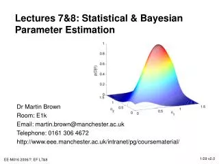
Lectures 7&8: Statistical & Bayesian Parameter Estimation. Dr Martin Brown Room: E1k Email: martin.brown@manchester.ac.uk Telephone: 0161 306 4672 http://www.eee.manchester.ac.uk/intranet/pg/coursematerial/. W7&8: Outline.

E N D
Lectures 7&8: Statistical & Bayesian Parameter Estimation Dr Martin Brown Room: E1k Email: martin.brown@manchester.ac.uk Telephone: 0161 306 4672 http://www.eee.manchester.ac.uk/intranet/pg/coursematerial/
W7&8: Outline • Parameter estimation is performed in a statistical framework. In these lectures, we’re going to look at: • L7 Statistical interpretation of least squares • Eigenvalue/eigenvector decomposition of the Hessian • Properties of the measurement noise/residual • Mean/variance of the parameter estimates • Prediction standard deviation (confidence) intervals • L8 Bayesian parameter estimation • Bayes formula & maximum likelihood estimation • Specifying prior knowledge • Prior parameter values and recursive estimation
W7&8: Resources • Core reading • Ljung: Chapter 7.4 • On-line: Chapters 5 & 6 • Norton: Chapters 5 • In these two lectures, we’ll be taking a statistical/Bayesian view of parameter estimation, looking at: • How the structure of the Hessian matrix XTX affects the condition of the estimation problem • Why the parameters are regarded as stochastic variables • What their estimates of mean and variance • How prior knowledge about their values can be incorporated using Bayesian theory
A “Centred” Quadratic Form • Note that the quadratic performance form can also be described by: • NB q and q are the unknown and least squares parameter vectors, which can easily be verified. Expanding and using the normal equations: • So when • This is equal to the sum of squares performance function. for some constant c ^
Hessian Matrix • The centred quadratic form is totally dependent on the form of the Hessian matrix H=XTX • The value is formed from the (weighed) parameter vector “error” size. • This is illustrated for f(q) & the contours of f(q).
Eigenvalue/Eigenvector Decomposition • For the DT electric circuit: • From this we note that cond(H) = 24.6. The matrix H determines the shape of the contours of f(). • When • The eigenvector/eigenvalue decomposition of H determines its properties/sensitivity in parameter space => =>
v2 v1 ^ q Eigenvalue/Eigenvector Picture • The eigenvectors form a basis for the parameter space. • The overall behaviour of f can be determined by looking at the orientations of vi and the corresponding eigenvalues. • When cond(H)1, it is easy to determine the optimal parameter estimate • When cond(H)>>1, small changes to the data can cause large changes in the optimal parameter estimates
Semi-positive Definite Hessian • H is semi-positive definite (all its eigenvalues are real and non-negative) • To prove this result, consider any vector x: • where z=Xx. If H is positive definite, all the eigenvalues are positive and the matrix is uniquely invertible. • Therefore if H is positive definite, we can uniquely estimate the optimal parameters, using normal form/least squares
Hessian Singularity & Normal Equations • To calculate the optimal parameter values, it is necessary to invert the Hessian matrix H: • This can only be achieved if H is full rank (H-1 exists) • Example: consider when there are two parameters in the model, but only one data point
^ q Quadratic Form and Singular Equations • In the diagram is can be seen that Df=0 for some changes in the parameter space (in the Null space of H or equivalently X) • The null space is spanned by the eigenvectors with corresponding eigenvalues=0. • If nN, then Xn = 0, Hn=0 and for this application • X(q+n) = Xq • There are an infinite number of optimal parameter vectors that are all equally ranked.
^ y(t) p(e) s 0 e Gaussian, Additive Measurement Noise r(t) “residual” x(t) Model q • We assume that the input signal x(t) is known exactly • We assume that the noise added to the exact output • We assume that the plant is linear and described by y = xTq+e • We assume that noise is zero-mean, Gaussian e ~ N(0,s2) - ^ + y(t) x(t) output measurement Plant q + + e(t)
Repeated Experiments • As stated earlier, the noise signal can be described by a zero mean, normal distribution • This states that if I perform a repeated experiment about a point, the mean value is the actual model output and the variance is the unobservable noise variance. e ~ N(0,s2) y ~ N(xTq,s2) Single variable y x
Parameter Estimate Statistics • As noted in Lab 5&6, if there exists random additive, measurement noise, and we create several data sets Di = {X, yi}i, then the estimated values for the parameter vectors, qi are different because the measured values are different, i.e. • The set of all estimated parameters forms a distribution centred on their true values where the variance/covariance is proportional to (XTX)-1, i.e. • In practice, this means that if we sample a random data set, the parameter estimates will, on average, be equal to their true values and the distribution of the estimates is related to the structure of (XTX)
Mean of Parameter Vector PDF Data Least squares parameter estimate • The mean of the least squares estimate is given by: • Which is simply the true, unknown parameters as required • Therefore the mean of the parameter vector PDF for the least squares solution is the true parameter vector. • The least squares estimate is not biased
Covariance of Parameter Vector PDF • The variance/covariance matrix of the least squares estimate is given by: • The parameter variance/covariance matrix depends on the variance of the unmeasurable noise and the inverse Hessian matrix
Example: Electrical Circuit (again!) • E(q) = [0.5 0.5]T • cov(q) = s2(XTX)-1 • Note the PDF(q|D) is Gaussian, because e is Gaussian Well determined l = 12.8 l = 0.52 poorly determined
Prediction Confidence Limits • As the model’s output is a linear combination of the estimated parameters, the output distribution is Gaussian • Therefore the model output represents the mean of the measured value (true response if noise is zero mean) • The variance/standard deviation of the prediction can be derived from
Example: Electrical Circuit • For each query point the error bars (standard deviation of the predictions) are calculated and used to “bracket” the prediction at +/- 2s, the 95% confidence intervals Note that the largest error bar (most uncertainty) occurs when t=2. When t=1, the error bar is zero, because the input is identically 0.
Bayesian Parameter Estimation Bayes rule can be used as a framework for parameter estimation: p(q|D) is the posterior conditional data distribution p(q) is the prior estimate of the parameter values p(D|q) is the data likelihood/conditional density function p(D) is the unconditional density function Remember, Bayes rule is derived from expressing the joint distribution in terms of the conditional and marginal distributions: But the two terms on the left hand side are the same, so:
Why use a Bayesian Framework? • There are three main reasons for interpreting parameter estimation within a Bayesian framework • Least squares estimation (maximum likelihood) is a simplified version of Bayesian learning • Bayesian learning allows the incorporation of prior knowledge about the parameter values • It can be used to motivate iterative/recurrent learning, where data is sequentially received and the parameters are updated after each time step • Learning corresponds to maximising p(q|D)p(D|q)p(q), i.e. selecting the parameter values for which there is the most evidence in the data
Likelihood Probability Density Function • The likelihood pdf is a conditional distribution and is given by • This is interpreted as “the probability of the data set being generated, given the parameter values”: Note: We wish to calculate the parameter values that maximise this quantity – its mean. Note that there is also a variance (see earlier)
Likelihood Function Assumptions • The output error signals are Gaussian independent and identically distributed (iid), they can be written as: • We want this value to be maximised (errors as small as possible), this can be achieved by minimising the negative log-likelihood (known as maximum likelihood estimation) Identically distributed means a common variance Independent means that the joint distribution is formed from the product of the individual distributions
Maximum Likelihood Estimation • To estimate the optimal parameter values, we wish to calculate the optimal parameter values that maximise this likelihood pdf • log() is a monotonic function, so we can maximise (s2 is positive constant): • multiplying by –1 is equivalent to minimising: • which is just the SSE performance function. Least squares parameter estimation is also known as maximium likelihood estimation because is maximises the likelihood distribution
Prior Parameter Distributions • To perform parameter estimation, we wish to select the parameter value that maximises the posterior • p(q|D)p(D|q)p(q) • i.e. the probability of the parameters given the data • p(q) represents a prior distribution (pdf) on the parameter values. It represents what “evidence” exists about the parameter estimates, before the data is observed/used. • The evidence could come from human beliefs about parameter values or from a previous data set • The use of prior evidence changes the estimated parameters when compared with just using the likelihood function to estimate their values
“every value is equally likely” p(q) q Uninformative Prior & MLE • If the prior knowledge about the parameters is not available, the parameter prior, p(q), is a flat pdf and is uninformative. • p(q) = c (infinitely small constant) and Bayesian parameter estimation is equivalent to maximum likelihood estimation, as • p(q|D) p(D|q)p(q) • = p(D|q) c • p(D|q) • As there is no prior evidence, all the information is contained in the training data set, and we simply have MLE.
Gaussian Prior • Another common prior is that there is some prior evidence for small parameter values p(q)exp(-lSiqi2), l>0 • Taking the negative log likelihood, we want to minimise • The Bayesian parameter estimate is given by • Note this is smaller than the LS estimate due to the prior. Sometimes known as regularization
Example: Electrical Circuit • Consider the normal least squares estimate and when we use Bayesian estimation with a Gaussian prior and l=0.5 • The performance of the two parameter estimates are roughly comparable, but some prior knowledge has been used to “shrink” the size of the estimated parameter values • As we’ll see later, typically large parameter values are a sign of over-fitting and poor generalisation
L7&8: Summary • Least squares parameter estimation is unbiased • The mean of the estimates is equal to the true values • E(q) = q • The variance/covariance of the parameter estimates is proportional to the inverse Hessian • Var(q) = s2(XTX)-1 • Bayes formula can be used for parameter estimation • Maximum likelihood is equivalent to least squares estimation when there is no prior knowledge (uninformative) • Simple prior knowledge about size of the parameter vector can be incorporated with Gaussian priors • Also used to motivate recursive estimation (next lectures) ^ ^
L7&8: Laboratory Session • Using the centred quadratic form, plot the performance function and its contours for the electrical circuit example • Calculate and plot the contours of the parameter estimate distribution (mean and cov) for the electrical circuit example • For each point in the model simulation, calculate both the prediction and the standard error associated with that prediction • Calculate the parameter estimates and residual vector when a regularized cost function is used with l=0.5, S26&27. • Re-calculate the parameter estimates and residual vector when l=0.1, 2.