Download

1 / 21
220 likes | 267 Views
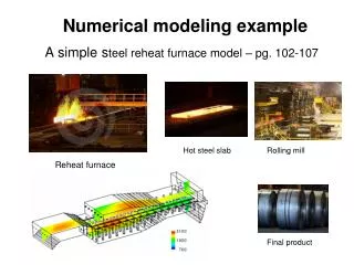
Numerical modeling example. A simple s teel reheat furnace model – pg. 99-116. Hot steel slab. Rolling mill. Reheat furnace. Final product. The implicit solution. Same equations with a minor change. The slab …. Dimensions: 10 m long 1 m wide 0.3 m thick. Steel Properties:

E N D
Numerical modeling example A simple steel reheat furnace model – pg. 99-116 Hot steel slab Rolling mill Reheat furnace Final product
The implicit solution Same equations with a minor change
The slab … • Dimensions: • 10 m long • 1 m wide • 0.3 m thick • Steel Properties: • k = 35 W/m-K • CP = 473.3 J/kg-K • r = 7820 kg/m3 • Model heat transfer through the 0.3 m dimension • “Convective” heat transfer based on a furnace gas temperature of 1400 K • Heat transfer symmetry on both sides of the slab; h = 200 W/m2-K • Centreline of the slab has a zero gradient boundary condition (q = 0)
Some computational considerations: No stability problems with this method. Time steps, t, and spatial steps, x, can be arbitrarily chosen by the user. Precision of the solution can be affected by the gird size (time and/or space) and this can be checked. We want to cover the slab region 0 < x < 0.15 m With x = 0.01 m we will require 15 cells
Same problem formulation and set up: Three different types of cells (implicit form): • Boundary next to the hot combustion gases – radiation modeled as a convective process. One cell only. • An array of interior cells. Many cells. • The centre plane boundary condition – plane of symmetry with q = 0. One cell only.
Cell adjacent to furnace gases: q = hA(T - TP) Accumulation within cell P = Input to cell P = TP evaluated at time step n+1 Output from cell P = TP and TE evaluated at time step n+1 Generation within cell P = 0 Accumulation = Input – Output + Generation
General interior cells: Accumulation within cell P = Input to cell P = TW and TP evaluated at time step n+1 Output from cell P = TP and TE evaluated at time step n+1 Generation in cell P = 0
Centreline Cell: Accumulation within cell P = TW and TP evaluated at time step n+1 Input to cell P = Output from cell P = 0 Generation in cell P = 0
The set of equations involve 15 cells with cell 1 adjacent to the furnace gases through to cell 15 on the centre symmetry plane of the slab Equation for cell 1: Equations for cell 2 – 14: Equation for cell 15:
Leads to a set of linear equations: A tridiagonal matrix
The vector of knowns (usually true for linear problems) The vector of unknowns
Diagonal elements of [A], Elements “banding” the diagonal coefficients in [A],
For ease of writing a computer code, define dimensionless groups: Diagonal elements of [A]: Banding elements of [A]:
Spreadsheet solution VBA (Excel add-in) format: 'Invoke TDMA to evaluate current temperatures ' Delta(1) = D(1) Y(1) = B(1) / Delta(1) For I = 2 To Number_of_Cells Delta(I) = D(I) - C(I) * E(I - 1) / Y(I - 1) Y(I) = (B(I) - C(I) * Y(I - 1)) / Delta(I) Next I X(Number_of_Cells) = Y(Number_of_Cells) For II = 2 To Number_of_Cells I = Number_of_Cells - II + 1 X(I) = Y(I) - E(I) * X(I + 1) / Delta(I) Next II ' 'Output from TDMA procedure is the solution vector X(I) Solver based on Tridiagonal Matrix Algorithm
Consider the system of equations: [A] x = b With 5 equations and 5 unknowns:
Decompose the original problem, [A] x = b To one of the form: [L][U] x = b Where[L] = and[U] = Lower triangular matrix Upper triangular matrix Need to find matrices [L] and [U] whose product equals original [A] matrix
With [A] x = band[L][U] x = b Let [U]x = ythen [L]y = b And b is known [L] = Solve for y by forward substitution in the system [L]y = b etc. i.e.
With a solution for y from [L]y = b Then solve for x from[U]x = y and y known [U] = Solve for x by backward substitution in the system [U]x = y i.e. x5 = y5 etc. And x is the solution to the original problem!!
A simpler case arises when the coefficient matrix [A] is tridiagonal: i.e. if [A] = [L] =
[U] = With backward substitution solution
'Invoke TDMA to evaluate current temperatures ‘Forward Substitution Code Delta(1) = D(1) Y(1) = B(1) / Delta(1) For I = 2 To Number_of_Cells Delta(I) = D(I) - C(I) * E(I - 1) / Y(I - 1) Y(I) = (B(I) - C(I) * Y(I - 1)) / Delta(I) Next I ‘Backward Substitution Code X(Number_of_Cells) = Y(Number_of_Cells) For II = 2 To Number_of_Cells I = Number_of_Cells - II + 1 X(I) = Y(I) - E(I) * X(I + 1) / Delta(I) Next II ' 'Output from TDMA procedure is the solution vector X(I)