Download

1 / 81
810 likes | 1.1k Views
Data Mining: Concepts and Techniques (3 rd ed.) — Chapter 8 —. 1. Classification: Basic Concepts Decision Tree Induction Bayes Classification Methods Rule-Based Classification Model Evaluation and Selection Techniques to Improve Classification Accuracy: Ensemble Methods Summary.

E N D
Data Mining: Concepts and Techniques(3rd ed.)— Chapter 8 — 1
Classification: Basic Concepts Decision Tree Induction Bayes Classification Methods Rule-Based Classification Model Evaluation and Selection Techniques to Improve Classification Accuracy: Ensemble Methods Summary Chapter 8. Classification: Basic Concepts 3
Supervised vs. Unsupervised Learning • Supervised learning (classification) • Supervision: The training data (observations, measurements, etc.) are accompanied by labels indicating the class of the observations • New data is classified based on the training set • Unsupervised learning(clustering) • The class labels of training data is unknown • Given a set of measurements, observations, etc. with the aim of establishing the existence of classes or clusters in the data
Prediction Problems: Classification vs. Numeric Prediction • Classification • predicts categorical class labels (discrete or nominal) • classifies data (constructs a model) based on the training set and the values (class labels) in a classifying attribute and uses it in classifying new data • Numeric Prediction • models continuous-valued functions, i.e., predicts unknown or missing values • Typical applications • Credit/loan approval: • Medical diagnosis: if a tumor is cancerous or benign • Fraud detection: if a transaction is fraudulent • Web page categorization: which category it is
Classification—A Two-Step Process • Model construction: describing a set of predetermined classes • Each tuple/sample is assumed to belong to a predefined class, as determined by the class label attribute • The set of tuples used for model construction is training set • The model is represented as classification rules, decision trees, or mathematical formulae • Model usage: for classifying future or unknown objects • Estimate accuracy of the model • The known label of test sample is compared with the classified result from the model • Accuracy rate is the percentage of test set samples that are correctly classified by the model • Test set is independent of training set (otherwise overfitting) • If the accuracy is acceptable, use the model to classify new data • Note: If the test set is used to select models, it is called validation (test) set
Training Data Classifier (Model) Process (1): Model Construction Classification Algorithms IF rank = ‘professor’ OR years > 6 THEN tenured = ‘yes’
Classifier Testing Data Unseen Data Process (2): Using the Model in Prediction (Jeff, Professor, 4) Tenured?
Chapter 8. Classification: Basic Concepts Classification: Basic Concepts Decision Tree Induction Bayes Classification Methods Rule-Based Classification Model Evaluation and Selection Techniques to Improve Classification Accuracy: Ensemble Methods Summary 9
age? <=30 overcast >40 31..40 student? credit rating? yes excellent fair no yes no yes no yes Decision Tree Induction: An Example • Training data set: Buys_computer • The data set follows an example of Quinlan’s ID3 (Playing Tennis) • Resulting tree:
Algorithm for Decision Tree Induction • Basic algorithm (a greedy algorithm) • Tree is constructed in a top-down recursive divide-and-conquer manner • At start, all the training examples are at the root • Attributes are categorical (if continuous-valued, they are discretized in advance) • Examples are partitioned recursively based on selected attributes • Test attributes are selected on the basis of a heuristic or statistical measure (e.g., information gain) • Conditions for stopping partitioning • All samples for a given node belong to the same class • There are no remaining attributes for further partitioning – majority voting is employed for classifying the leaf • There are no samples left
Brief Review of Entropy m = 2
Attribute Selection Measure: Information Gain (ID3/C4.5) • Select the attribute with the highest information gain • Let pi be the probability that an arbitrary tuple in D belongs to class Ci, estimated by |Ci, D|/|D| • Expected information (entropy) needed to classify a tuple in D: • Information needed (after using A to split D into v partitions) to classify D: • Information gained by branching on attribute A
Class P: buys_computer = “yes” Class N: buys_computer = “no” means “age <=30” has 5 out of 14 samples, with 2 yes’es and 3 no’s. Hence Similarly, Attribute Selection: Information Gain
Computing Information-Gain for Continuous-Valued Attributes • Let attribute A be a continuous-valued attribute • Must determine the best split point for A • Sort the value A in increasing order • Typically, the midpoint between each pair of adjacent values is considered as a possible split point • (ai+ai+1)/2 is the midpoint between the values of ai and ai+1 • The point with the minimum expected information requirement for A is selected as the split-point for A • Split: • D1 is the set of tuples in D satisfying A ≤ split-point, and D2 is the set of tuples in D satisfying A > split-point
Gain Ratio for Attribute Selection (C4.5) • Information gain measure is biased towards attributes with a large number of values • C4.5 (a successor of ID3) uses gain ratio to overcome the problem (normalization to information gain) • GainRatio(A) = Gain(A)/SplitInfo(A) • Ex. • gain_ratio(income) = 0.029/1.557 = 0.019 • The attribute with the maximum gain ratio is selected as the splitting attribute
Gini Index (CART, IBM IntelligentMiner) • If a data set D contains examples from n classes, gini index, gini(D) is defined as where pj is the relative frequency of class j in D • If a data set D is split on A into two subsets D1 and D2, the gini index gini(D) is defined as • Reduction in Impurity: • The attribute provides the smallest ginisplit(D) (or the largest reduction in impurity) is chosen to split the node (need to enumerate all the possible splitting points for each attribute)
Computation of Gini Index • Ex. D has 9 tuples in buys_computer = “yes” and 5 in “no” • Suppose the attribute income partitions D into 10 in D1: {low, medium} and 4 in D2 Gini{low,high} is 0.458; Gini{medium,high} is 0.450. Thus, split on the {low,medium} (and {high}) since it has the lowest Gini index • All attributes are assumed continuous-valued • May need other tools, e.g., clustering, to get the possible split values • Can be modified for categorical attributes
Comparing Attribute Selection Measures • The three measures, in general, return good results but • Information gain: • biased towards multivalued attributes • Gain ratio: • tends to prefer unbalanced splits in which one partition is much smaller than the others • Gini index: • biased to multivalued attributes • has difficulty when # of classes is large • tends to favor tests that result in equal-sized partitions and purity in both partitions
Other Attribute Selection Measures • CHAID: a popular decision tree algorithm, measure based on χ2 test for independence • C-SEP: performs better than info. gain and gini index in certain cases • G-statistic: has a close approximation to χ2 distribution • MDL (Minimal Description Length) principle (i.e., the simplest solution is preferred): • The best tree as the one that requires the fewest # of bits to both (1) encode the tree, and (2) encode the exceptions to the tree • Multivariate splits (partition based on multiple variable combinations) • CART: finds multivariate splits based on a linear comb. of attrs. • Which attribute selection measure is the best? • Most give good results, none is significantly superior than others
Overfitting and Tree Pruning • Overfitting: An induced tree may overfit the training data • Too many branches, some may reflect anomalies due to noise or outliers • Poor accuracy for unseen samples • Two approaches to avoid overfitting • Prepruning: Halt tree construction early̵ do not split a node if this would result in the goodness measure falling below a threshold • Difficult to choose an appropriate threshold • Postpruning: Remove branches from a “fully grown” tree—get a sequence of progressively pruned trees • Use a set of data different from the training data to decide which is the “best pruned tree”
Enhancements to Basic Decision Tree Induction • Allow for continuous-valued attributes • Dynamically define new discrete-valued attributes that partition the continuous attribute value into a discrete set of intervals • Handle missing attribute values • Assign the most common value of the attribute • Assign probability to each of the possible values • Attribute construction • Create new attributes based on existing ones that are sparsely represented • This reduces fragmentation, repetition, and replication
Classification in Large Databases • Classification—a classical problem extensively studied by statisticians and machine learning researchers • Scalability: Classifying data sets with millions of examples and hundreds of attributes with reasonable speed • Why is decision tree induction popular? • relatively faster learning speed (than other classification methods) • convertible to simple and easy to understand classification rules • can use SQL queries for accessing databases • comparable classification accuracy with other methods • RainForest (VLDB’98 — Gehrke, Ramakrishnan & Ganti) • Builds an AVC-list (attribute, value, class label)
Scalability Framework for RainForest • Separates the scalability aspects from the criteria that determine the quality of the tree • Builds an AVC-list: AVC (Attribute, Value, Class_label) • AVC-set (of an attribute X ) • Projection of training dataset onto the attribute X and class label where counts of individual class label are aggregated • AVC-group (of a node n ) • Set of AVC-sets of all predictor attributes at the node n
Rainforest: Training Set and Its AVC Sets Training Examples AVC-set on Age AVC-set on income AVC-set on credit_rating AVC-set on Student
BOAT (Bootstrapped Optimistic Algorithm for Tree Construction) Use a statistical technique called bootstrapping to create several smaller samples (subsets), each fits in memory Each subset is used to create a tree, resulting in several trees These trees are examined and used to construct a new tree T’ It turns out that T’ is very close to the tree that would be generated using the whole data set together Adv: requires only two scans of DB, an incremental alg. 26
Data Mining: Concepts and Techniques Presentation of Classification Results
Data Mining: Concepts and Techniques Visualization of a Decision Tree in SGI/MineSet 3.0
Data Mining: Concepts and Techniques Interactive Visual Mining by Perception-Based Classification (PBC)
Chapter 8. Classification: Basic Concepts Classification: Basic Concepts Decision Tree Induction Bayes Classification Methods Rule-Based Classification Model Evaluation and Selection Techniques to Improve Classification Accuracy: Ensemble Methods Summary 30
Bayesian Classification: Why? • A statistical classifier: performs probabilistic prediction, i.e., predicts class membership probabilities • Foundation: Based on Bayes’ Theorem. • Performance: A simple Bayesian classifier, naïve Bayesian classifier, has comparable performance with decision tree and selected neural network classifiers • Incremental: Each training example can incrementally increase/decrease the probability that a hypothesis is correct — prior knowledge can be combined with observed data • Standard: Even when Bayesian methods are computationally intractable, they can provide a standard of optimal decision making against which other methods can be measured
Bayes’ Theorem: Basics • Total probability Theorem: • Bayes’ Theorem: • Let X be a data sample (“evidence”): class label is unknown • Let H be a hypothesis that X belongs to class C • Classification is to determine P(H|X), (i.e., posteriori probability): the probability that the hypothesis holds given the observed data sample X • P(H) (prior probability): the initial probability • E.g., X will buy computer, regardless of age, income, … • P(X): probability that sample data is observed • P(X|H) (likelihood): the probability of observing the sample X, given that the hypothesis holds • E.g.,Given that X will buy computer, the prob. that X is 31..40, medium income
Prediction Based on Bayes’ Theorem • Given training dataX, posteriori probability of a hypothesis H, P(H|X), follows the Bayes’ theorem • Informally, this can be viewed as posteriori = likelihood x prior/evidence • Predicts X belongs to Ci iff the probability P(Ci|X) is the highest among all the P(Ck|X) for all the k classes • Practical difficulty: It requires initial knowledge of many probabilities, involving significant computational cost
Classification Is to Derive the Maximum Posteriori • Let D be a training set of tuples and their associated class labels, and each tuple is represented by an n-D attribute vector X = (x1, x2, …, xn) • Suppose there are m classes C1, C2, …, Cm. • Classification is to derive the maximum posteriori, i.e., the maximal P(Ci|X) • This can be derived from Bayes’ theorem • Since P(X) is constant for all classes, only needs to be maximized
Naïve Bayes Classifier • A simplified assumption: attributes are conditionally independent (i.e., no dependence relation between attributes): • This greatly reduces the computation cost: Only counts the class distribution • If Ak is categorical, P(xk|Ci) is the # of tuples in Ci having value xk for Ak divided by |Ci, D| (# of tuples of Ci in D) • If Ak is continous-valued, P(xk|Ci) is usually computed based on Gaussian distribution with a mean μ and standard deviation σ and P(xk|Ci) is
Naïve Bayes Classifier: Training Dataset Class: C1:buys_computer = ‘yes’ C2:buys_computer = ‘no’ Data to be classified: X = (age <=30, Income = medium, Student = yes Credit_rating = Fair)
Naïve Bayes Classifier: An Example • P(Ci): P(buys_computer = “yes”) = 9/14 = 0.643 P(buys_computer = “no”) = 5/14= 0.357 • Compute P(X|Ci) for each class P(age = “<=30” | buys_computer = “yes”) = 2/9 = 0.222 P(age = “<= 30” | buys_computer = “no”) = 3/5 = 0.6 P(income = “medium” | buys_computer = “yes”) = 4/9 = 0.444 P(income = “medium” | buys_computer = “no”) = 2/5 = 0.4 P(student = “yes” | buys_computer = “yes) = 6/9 = 0.667 P(student = “yes” | buys_computer = “no”) = 1/5 = 0.2 P(credit_rating = “fair” | buys_computer = “yes”) = 6/9 = 0.667 P(credit_rating = “fair” | buys_computer = “no”) = 2/5 = 0.4 • X = (age <= 30 , income = medium, student = yes, credit_rating = fair) P(X|Ci) : P(X|buys_computer = “yes”) = 0.222 x 0.444 x 0.667 x 0.667 = 0.044 P(X|buys_computer = “no”) = 0.6 x 0.4 x 0.2 x 0.4 = 0.019 P(X|Ci)*P(Ci) : P(X|buys_computer = “yes”) * P(buys_computer = “yes”) = 0.028 P(X|buys_computer = “no”) * P(buys_computer = “no”) = 0.007 Therefore, X belongs to class (“buys_computer = yes”)
Avoiding the Zero-Probability Problem • Naïve Bayesian prediction requires each conditional prob. be non-zero. Otherwise, the predicted prob. will be zero • Ex. Suppose a dataset with 1000 tuples, income=low (0), income= medium (990), and income = high (10) • Use Laplacian correction (or Laplacian estimator) • Adding 1 to each case Prob(income = low) = 1/1003 Prob(income = medium) = 991/1003 Prob(income = high) = 11/1003 • The “corrected” prob. estimates are close to their “uncorrected” counterparts
Naïve Bayes Classifier: Comments • Advantages • Easy to implement • Good results obtained in most of the cases • Disadvantages • Assumption: class conditional independence, therefore loss of accuracy • Practically, dependencies exist among variables • E.g., hospitals: patients: Profile: age, family history, etc. Symptoms: fever, cough etc., Disease: lung cancer, diabetes, etc. • Dependencies among these cannot be modeled by Naïve Bayes Classifier • How to deal with these dependencies? Bayesian Belief Networks (Chapter 9)
Chapter 8. Classification: Basic Concepts Classification: Basic Concepts Decision Tree Induction Bayes Classification Methods Rule-Based Classification Model Evaluation and Selection Techniques to Improve Classification Accuracy: Ensemble Methods Summary 40
Using IF-THEN Rules for Classification • Represent the knowledge in the form of IF-THEN rules R: IF age = youth AND student = yes THEN buys_computer = yes • Rule antecedent/precondition vs. rule consequent • Assessment of a rule: coverage and accuracy • ncovers = # of tuples covered by R • ncorrect = # of tuples correctly classified by R coverage(R) = ncovers /|D| /* D: training data set */ accuracy(R) = ncorrect / ncovers • If more than one rule are triggered, need conflict resolution • Size ordering: assign the highest priority to the triggering rules that has the “toughest” requirement (i.e., with the most attribute tests) • Class-based ordering: decreasing order of prevalence or misclassification cost per class • Rule-based ordering (decision list): rules are organized into one long priority list, according to some measure of rule quality or by experts
age? <=30 >40 31..40 student? credit rating? yes excellent fair no yes no yes no yes Rule Extraction from a Decision Tree • Rules are easier to understand than large trees • One rule is created for each path from the root to a leaf • Each attribute-value pair along a path forms a conjunction: the leaf holds the class prediction • Rules are mutually exclusive and exhaustive • Example: Rule extraction from our buys_computer decision-tree IF age = young AND student = no THEN buys_computer = no IF age = young AND student = yes THEN buys_computer = yes IF age = mid-age THEN buys_computer = yes IF age = old AND credit_rating = excellent THEN buys_computer = no IF age = old AND credit_rating = fair THEN buys_computer = yes
Rule Induction: Sequential Covering Method • Sequential covering algorithm: Extracts rules directly from training data • Typical sequential covering algorithms: FOIL, AQ, CN2, RIPPER • Rules are learned sequentially, each for a given class Ci will cover many tuples of Ci but none (or few) of the tuples of other classes • Steps: • Rules are learned one at a time • Each time a rule is learned, the tuples covered by the rules are removed • Repeat the process on the remaining tuples until termination condition, e.g., when no more training examples or when the quality of a rule returned is below a user-specified threshold • Comp. w. decision-tree induction: learning a set of rules simultaneously
Sequential Covering Algorithm while (enough target tuples left) generate a rule remove positive target tuples satisfying this rule Examples covered by Rule 2 Examples covered by Rule 1 Examples covered by Rule 3 Positive examples
Rule Generation • To generate a rule while(true) find the best predicate p if foil-gain(p) > threshold then add p to current rule else break A3=1 A3=1&&A1=2 A3=1&&A1=2 &&A8=5 Positive examples Negative examples
How to Learn-One-Rule? • Start with the most general rule possible: condition = empty • Adding new attributes by adopting a greedy depth-first strategy • Picks the one that most improves the rule quality • Rule-Quality measures: consider both coverage and accuracy • Foil-gain (in FOIL & RIPPER): assesses info_gain by extending condition • favors rules that have high accuracy and cover many positive tuples • Rule pruning based on an independent set of test tuples Pos/neg are # of positive/negative tuples covered by R. If FOIL_Prune is higher for the pruned version of R, prune R
Chapter 8. Classification: Basic Concepts Classification: Basic Concepts Decision Tree Induction Bayes Classification Methods Rule-Based Classification Model Evaluation and Selection Techniques to Improve Classification Accuracy: Ensemble Methods Summary 47
Model Evaluation and Selection • Evaluation metrics: How can we measure accuracy? Other metrics to consider? • Use validation test set of class-labeled tuples instead of training set when assessing accuracy • Methods for estimating a classifier’s accuracy: • Holdout method, random subsampling • Cross-validation • Bootstrap • Comparing classifiers: • Confidence intervals • Cost-benefit analysis and ROC Curves 48
Classifier Evaluation Metrics: Confusion Matrix Confusion Matrix: Example of Confusion Matrix: • Given m classes, an entry, CMi,j in a confusion matrix indicates # of tuples in class i that were labeled by the classifier as class j • May have extra rows/columns to provide totals 49
Classifier Evaluation Metrics: Accuracy, Error Rate, Sensitivity and Specificity • Classifier Accuracy, or recognition rate: percentage of test set tuples that are correctly classified Accuracy = (TP + TN)/All • Error rate:1 –accuracy, or Error rate = (FP + FN)/All • Class Imbalance Problem: • One class may be rare, e.g. fraud, or HIV-positive • Significant majority of the negative class and minority of the positive class • Sensitivity: True Positive recognition rate • Sensitivity = TP/P • Specificity: True Negative recognition rate • Specificity = TN/N 50