Download
1 / 18
180 likes | 308 Views
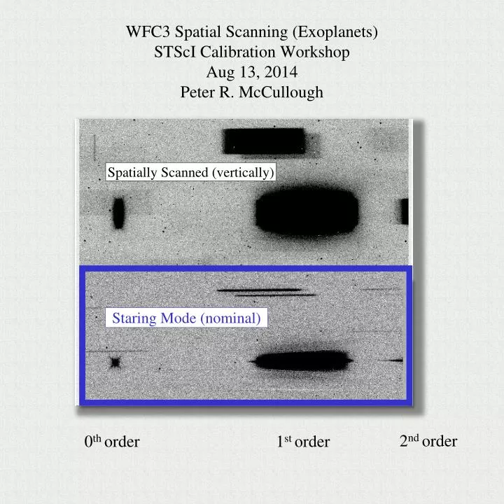
WFC3 Spatial Scanning ( Exoplanets ) STScI Calibration Workshop Aug 13, 2014 Peter R. McCullough. Spatially Scanned (vertically). H 2 O. H 2 O. Staring Mode (nominal). 2 nd order. 0 th order. 1 st order. Build it and they will come…. Benneke & Crossfield et al. 2014-15, 100+ orbits.

E N D
WFC3 Spatial Scanning (Exoplanets)STScI Calibration WorkshopAug 13, 2014Peter R. McCullough Spatially Scanned (vertically) H2O H2O Staring Mode (nominal) 2nd order 0th order 1st order
Build it and they will come… Benneke & Crossfield et al. 2014-15, 100+ orbits Bean et al. 2013-14, 100+ orbits
Scan ? Spatially Scanned (vertically) Who ? • McCullough & MacKenty (ISR WFC3-2012-08) What ? • Spatial scanning means moving the telescope (HST) during an exposure, in this case perpendicular to the dispersion of the spectrum. • HST can scan at any rate from 0 to 7.8 arcsec s-1. The scan rate determines the effective exposure time. Where ? • Hubble/WFC3 (also now on Spitzer but not spectroscopically) When ? • Since 2011 (and S.O.P. in the old days of photographic plates) Why ? • Spatial scanning increases the number of photons recorded by a large factor because spatial scanning reduces overheads considerably. For each detector preparation-readout cycle, we obtain ~100 spectra (well-exposed rows on the detector) instead of just 1. • Spatial scanning is most useful for bright stars (H < 10 mag). • For very bright stars (H ~ 6 mag) such as HD 189733 and HD 209458, spatial scanning enables observations that otherwise would saturate the detector even before the exposure begins. • Spatial scanning has enable the “greatest hits” science by increasing the S/N of exoplanet spectroscopy by factors of a few. How (to analyze the data) ? • This Presentation … 0th 1st 2nd Staring Mode (nominal)
WFC3: Precision Infrared Spectrophotometry with Spatial Scans of HD 189733b and Vega P. R. McCullough (STScI & JHU), Nicolas Crouzet (STScI & Dunlap Inst.), Drake Deming (U. MD), Nikku Madhusudhan (Yale & Cambridge), & Susana E. Deustua (STScI) The Wide Field Camera 3 (WFC3) on the Hubble Space Telescope (HST) now routinely provides near-infrared spectroscopy of transiting extrasolar planet atmospheres with better than ~50 ppm precision per 0.05-micron resolution bin per transit, for sufficiently bright host stars. Two improvements of WFC3 (the detector) and HST (the spatial scanning technique) have made transiting planet spectra more sensitive and more repeatable than was feasible with NICMOS. In addition, the data analysis is much simpler with WFC3 than with NICMOS. We present time-series spectra of HD 189733b from 1.1 to 1.7 microns in transit and eclipse with fidelity similar to that of the WFC3 transit spectrum of HD 209458b (Deming et al. 2013). In a separate program, we obtained scanned infrared spectra of the bright star, Vega, thereby extending the dynamic range of WFC3 to ~26 magnitudes! Analysis of these data will affect the absolute spectrophotometric calibration of the WFC3, placing it on an SI traceable scale From top to bottom, transit spectra of HD 209458b and XO-1b (Deming et al. 2013), GJ436b (Knutson et al. 2013), and GJ 1214b (Kriedberg et al. 2014). The number of transits and estimated uncertainty in each R~70 spectral channel are listed. We scanned the gas giant exoplanet HD 189733b with WFC3 in June, 2013. Its transit spectrum (blue data points, black model) shows water vapor features at 1.2 microns and 1.4 microns similar to those of HD 209458b as reported by Deming et al. (2013) and commensurate with a solar-abundance clear atmosphere (McCullough et al. 2014). Its eclipse spectrum (blue data points, black model) is flat and its molecular features are lower contrast than similar models predict (Crouzet et al. 2014). • Spatial scanning means moving the telescope (HST) during an exposure, in this case perpendicular to the dispersion of the spectrum. • HST can scan at any rate from 0 to 7.8 arcsec s-1. The scan rate determines the effective exposure time. • Spatial scanning increases the number of photons recorded by a large factor because spatial scanning reduces overheads considerably. For each detector preparation-readout cycle, we obtain ~100 spectra (well-exposed rows on the detector) instead of just 1. • Spatial scanning is most useful for bright stars (H < 10 mag). • For very bright stars (H ~ 6 mag) such as HD 189733 and HD 209458, spatial scanning enables observations that otherwise would saturate the detector even before the exposure begins. • Spatial scanning has enable the “greatest hits” science in the sidebar (at far right) by increasing the S/N of exoplanet spectroscopy by factors of a few. Abstract WFC3 Spatial Scans “Greatest Hits” Spatial Scans: How and Why HD 189733b Spatially Scanned (vertically) HD 209458b, H=6.4, 1 transit, 36 ppm 0th 1st 2nd HD 189733b, H=5.6, 1 transit, 69 ppm Staring Mode (nominal) XO-1b, H=9.6, 1 transit, 96 ppm HD 189733b, H=5.6, 1 eclipse, 57 ppm GJ 436b, H=6.3, 4 transits, 40 ppm Spectra of Vega for the -1st orders of the two WFC3 IR grisms (Deustua et al. 2014). Solid lines represent “slower” scan rates (< 5 ”s-1); dashed lines represent faster scans (> 7 ”s-1). Left: at 24 Å/pix, Pa is just visible at 1.09 microns, and Pa at 1.05 microns. Right: at 46 Å/pix, Paschen is the dip at 1.28 microns, and the series of features between 1.6 and 1.7 microns are Br 13,12, 11. Vega GJ 1214b, H=9.1, 12 transits, 28 ppm The spatially scanned spectrum of the star GJ1214 is labeled with its 0th, 1st, and 2nd order light and compared to a nominal staring-mode slitless spectrum of the same field (blue outlined inset). The images are 512 columns wide, of the detector’s 1024. The scan was 40 pixels high. (4.8 arcsec). References Crouzet et al. 2014, ApJ, in prep. Deustua et al. 2014, in prep. Deming et al. 2013, ApJ, 774, 95 Knutson et al. 2014, Nature, 505, 66 Kreidberg et al. 2014, Nature. 505, 69 McCullough et al. 2014, ApJ, in prep. AAS Conference, Jan 8, 2014, Washington D.C. USA, Poster 347.21
Spatial Scanning with HST for Exoplanet Transit Spectroscopy and other High Dynamic Range Observations P. R. McCullough & J. MacKenty (STScI) In this test, we trailed the star GJ 1214 across the WFC3 IR detector repeatedlyat a rate of 0.1 arcsec s-1perpendicular to the dispersion of the G141 grism. By coincidence we observed for 15 minutes during the egress of the transiting extrasolar planet GJ 1214b. The utility of scanning for the UVIS grism will be limited to 200 nm to 400 nm, due to order overlap longer than 400 nm. INFRARED: In one test, we trailed the star P330E across the WFC3 IR detector repeatedly, with rates of 1, 1, and 0.5 arcsec s-1 respectively. Photometry (above), integrated transverse to each of the three trails, show intermittent oscillations with ~3% amplitude at ~1.3 Hz, due to image motion or “jitter” during the scans. The 2nd and 3rd trails have been offset vertically by 0.1 and 0.2 for clarity. According to Bradley (2011), at these scanning rates, the jitter measured by the Fine Guidance Sensor (FGS) in closed-loop guiding was not significantly different than for nominal staring-mode operation of HST, ~0.0035 arcsec rms in each of two orthogonal axes. The power spectrum of the jitter contains peaks at 6.2, 3.3, 2.9, 1.3, and some less than 1 Hz, caused by the NICMOS cooling system, the high gain antenna, the aperture door, and the solar arrays. The photometric oscillations are commensurate with the jitter. For example, consider the time-dependent position of the star D(t) = V0t + A sin ω t, where the first term is the uniform scan rate and the second term models the oscillatory jitter. The velocity is V(t) = V0 + A ω cos ω t, and hence the variability of the time for a star to cross a pixel, which determines the photometric variability along a scan, is sinusoidal with 3% amplitude, i.e. A ω / V0 = 0.03 for A = 0.0035 arcsec, ω = 2π(1.3 Hz), and V0= 1 arcsec s-1. For a detector well-calibrated to linearity, oscillations of the sort described above should not affect the photometric integral over the entire scan, in principle, except for the jitter’s effect on the precise location (and hence time) of the start and finish of each scan. For IR imaging, the latter exception can be made negligible by scanning parallel to the fast-read direction of the IR readout., i.e. “horizontally.” Ultraviolet-visible (UVIS): In another test, we trailed the star GJ 1214 repeatedly across the same pixels of the UVIS detector at a rate of 1 arcsec s-1 for eight 5-s F814W exposures. Integrated over the entire 125-pixel long scan, the photometric repeatability was 4.0 mmag rms, or 40% greater than the quadrature sum of Poisson noise (1.1 mmag) and shutter noise (2.7 mmag). For the latter we adopted 12 milliseconds rms of shutter jitter per 5-s exposure (Hilbert 2009). The overheads per WFC3 UVIS-M512C-SUB exposure in our tests ranged from 58 s to 92 s; the 58 s value was the most common, and it was the same for staring mode or scans. Scanned Imaging Scanned Spectroscopy The spatially scanned spectrum of the star GJ1214 is labeled with its 0th, 1st, and 2nd order light and compared to a nominal staring-mode slitless spectrum of the same field (blue outlined inset). The images are 512 columns wide, of the detector’s 1024. The scan was 40 pixels high. (4.8 arcsec). Spatially Scanned (vertically) ABSTRACT We are reviving an old technique of spatially scanning the telescope to improve observations, in this case with the Hubble Space Telescope's Wide Field Camera 3 (HST WFC3). Spatial scanning will turn stars into well-defined streaks on the detector, or, for example, spread a stellar spectrum perpendicular to its dispersion. There are at least two motivations for implementing such a capability: 1) reducing the fraction of overhead in observations of very bright stars such as those suitable for spectral characterization of transiting planets, and 2) enabling observations of very bright primary calibrators that otherwise would saturate the IR detector. We report results (McCullough & MacKenty 2011) from two engineering tests in which a star was imaged with WFC3 IR under various parameterizations of HST's scanning speed and orientation, and with or without a grism in place. 0th 1st 2nd Staring Mode (nominal) Why would we do this? CONCLUSION: It works! The re-introduction of spatial scanning to HST has been demonstrated for WFC3 IR and UVIS.We expect that the two primary motivations (see Abstract) are achievable. POTENTIAL APPLICATIONS We anticipate a number of potential applications for spatial scanning with HST. You are encouraged to discuss possibilities with us. Here are a few. For transit spectroscopy of exoplanets with WFC3, spatial scanning could increase the number of IR photons recorded by a factor of 10 for a star like GJ 1214 (H=9.09 mag), because spatial scanning reduces overheads considerably. For even brighter stars such as HD 189733, spatial scanning will enable observations that otherwise would be compromised by pre-exposure saturation of the IR detector that lacks a physical shutter. For a slitless stellar spectrum, one requires a wavelength-dependent flat field, but now we can get what we want directly, in orbit, using a spatially-scanned spectrum of a reference star for calibration. If we can increase the maximum scan rate to 2 arcsec s-1, the primary calibrator star Vega will not saturate the IR detector pixels with the G141 grism in its -1st order, which is ~4.6 mag less efficient than the +1storder (Kuntschner et al. 2011). Similarly, in imaging mode, spatial scanning should permit unsaturated IR photometry of calibrators without concern that the star “burns in,” i.e. gradually appears to brighten (by ~0.5%) with time due to its own electronic “after images.” For example, a G2 V star, with H = 9.9 mag, scanned at 1 arcsec s-1and imaged with the F125W filter will be marginally below saturation of the IR detector. TWO TESTS We executed two on-orbit tests under HST program 12325, one on 2011-03-24 (IR imaging only) and the other 2011-04-18 (UVIS imaging & IR spectroscopy). The first test proved that we can scan a star across the IR detector in a straight line at a constant rate with well-defined starting and finishing positions. The second test demonstrated 1) the same capability for the UVIS detector (perhaps indicating an adjustment is needed in the synchronization with the UVIS channel), 2) that scanning works also for spectroscopy using the G141 grism with the IR detector, and 3) measured the operational overheads associated with a time series of scans. SPECIFYING A SCAN Referring to the figure below, the observer must define the scan rate, scan orient angle α, and scan direction (forward, meaning from a to b, or reverse, from b to a). Currently the scan rate must be less than 1 arcsec s-1 (limited by flight software parameters), but we are investigating if it can be increased to 7.84 arcsec s-1 (limited by gyros). For a given scan rate, the scan length on the detector is determined by the effective exposure time, which depends on both the commanded exposure time and whether the star is scanning “upstream” or “downstream” of the IR detector’s raster-scanned readout. Acknowledgments Zach Berta (Harvard), the P.I. of HST program 12251, “The first characterization of a Super-Earth Atmosphere,” gracious agreed to our request to use GJ 1214 also for our 2nd test. Many persons, especially Merle Reinhart, Alan Welty, and William “Bill” Januszewski (STScI) helped plan the observations. Art Bradley (SSES) and Mike Wenz (GSFC) provided FGS data and analysis. Many persons, especially Adam Reiss and Susana Deustua, suggested applications for spatial scanning. References Bradley, A. 2011, Spacecraft System Engineering Services, private communication of unpublished report “FGS Vehicle Scan (#52 Command) On-Orbit Test of 2011:083” Hilbert, B. 2009, WFC3 ISR 2009-25, “WFC3 SMOV Program 11427: UVIS Channel Shutter Shading” Kuntschner et al. 2011, WFC3 ISR 2011-5, “Revised Flux Calibration of the WFC3 G102 and G141 grisms” McCullough & MacKenty, J. 2011, WFC3 ISR 2011-NN, in preparation The overheads per WFC3 IR exposure in a series in our tests were 19 s, 40 s, and 67 s, for nominal staring-mode, scanning mode (forward then reverse), and scanning mode (forward every time). The scans were at 1 arcsec s-1. Exploring Strange New Worlds, May 1-6, 2011, Flagstaff AZ USA
Calibration of Scanned Spectraincomplete bibliography McCullough et al. (2012) McCullough & MacKenty (2012) [ Berta et al. (2012), GJ 1214 transits (staring) ] Deming et al. (2013), XO-1 & HD 209458 transits Swain et al. (2013)* Kreidberget al. (2014a), GJ 1214 transit Knutson et al. (2014), GJ 436 transit McCullough et al. (2014), HD 189733 transit Crouzetet al. (2014) in press, HD 189733 eclipse Stevenson et al. (2014) in press, WASP-43 phase curves Kreidberg et al. (2014b) submitted, WASP-43 transits Unrefereed * Alternative view
Caveat Emptor A contradictory view is available, http://arxiv.org/abs/1311.3934 : Comparing the WFC3 IR Grism Stare and Spatial-Scan Observations for Exoplanet Characterization, Mark R. Swain, Pieter Deroo, Kiri L. Wagstaff (15 Nov 2013)* We report on a detailed study of the measurement stability for WFC3 IR grism stare and spatial scan observations. The excess measurement noise for both modes is established by comparing the observed and theoretical measurement uncertainties. We find that the stare-mode observations produce differential measurements that are consistent and achieve ∼1.3 times photon-limited measurement precision. In contrast, the spatial-scan mode observations produce measurements which are inconsistent, non-Gaussian, and have higher excess noise corresponding to ∼2 times the photon-limited precision. The inferior quality of the spatial scan observations is due to spatial-temporal variability in the detector performance which we measure and map. The non-Gaussian nature of spatial scan measurements makes the use of χ2 and the determination of formal confidence intervals problematic and thus renders the comparison of spatial scan data with theoretical models or other measurements difficult. With better measurement stability and no evidence for non-Gaussianity, stare mode observations offer a significant advantage for characterizing transiting exoplanet systems. * Reiterated March 2014 at Caltech JWST-exoplanets meeting
HD 189733b transit & eclipse Three permutations of McCullough, Crouzet, Madhusudhan, Deming 2014 HD 209458b and XO-1bDeming et al. 2013 HD 209458b, H=6.4 1 transit, 36 ppm H2O H2O XO-1b, H=9.6 1 transit, 96 ppm
WASP-43bStevenson, Bean et al. 2014 H2O H2O (full phase, near Eclipse) (new phase, near transit)
Direct Image We use the direct image mainly to verify the positions and fluxes of neighboring stars in the field of view.
Steps of Calibration • Discard data from first orbit (optional) of four or five orbits per visit (per transit or eclipse). • Start with IMA files (or make your own from RAW files (tedious) ) • Dark-corrected • Nonlinearity corrected • Flagged-pixel masks (optional) • Sort into Forward & Reverse scanning directions • POSTARG2 keyword is helpful • Form forward differences of consecutive reads. • Divide by flat field • It’s useful to ID bad pixel & cosmic ray hits. • We use F139M but it hardly matters because … • We eventually divide by the best-possible self-calibrated “flat,” derived from out-of-transit data before and after the transit event. • Interpolate values for bad pixels and cosmics. • Measure and subtract sky value from each image. • Sum over appropriate rows and columns to convert 2-D spectrum to 1-D spectrum. • Shift/interpolate 1-D spectra to common grid (optional). • Calibrate column wavelength. • Smooth 1-D spectra (optional; cf. Deming et al. 2013). Of course, smoothing reduces noise and spectral resolution (see McCullough et al. 2014 for factor (0.817) relating box-car & Gaussian smoothing). • Form exoplanet spectrum = (OUT - IN)/OUT = 1 – IN/OUT
Wiggles, Drifts and Smoothing Swain 2013 ArXiv preprint
Wavelength Calibration In McCullough et al. 2014, we used a calibrated, ground-based, higher-resolution spectrum of a similar star, and transformed it iteratively (by smoothing, shifting, stretching, re-binning) until it best matched our observed WFC3 stellar spectrum. Others (e.g. Bean, Kriedberg& Stevenson) have used proper WFC3 distortion-parameterized wavelength calibration files, and the direct image to set the zero point. This is tedious and prone to bookkeeping blunders. It may be necessary for very long scans (>> 100 rows) due to distortion. On the other hand, because we generally use 4-column-wide bins in final spectra, small shifts due to distortion hardly matter.
Limb Darkening & Star Spots The presumed limb-darkening model parameters do not affect the differential transmission spectrum much at all: its shape and relative heights of features remain the same. However, limb-darkening critically affects the white-light transit depth, and hence comparisons with other pan-chromatic observations. The white-light transit depth also is affected by star spots away from the transit chord (especially for HD 189733b).
Caveat Emptor: rawima Zero signal array (522x522) Last ima.fits Order 1 Order 2 Star A 1800 e 38000 e 800 e Star B Scan direction Ragged edge of “if” statement within signal box at ~260 e/pixel in 0th read.
Summary • Transiting exoplanet spectra require very high S/N (10,000:1 or more). • Scanning records 10-100 times more photons than staring. • Scanning prevents saturation of very bright stars. • Analysis of scanned spectra is easier than that of staring-mode spectra. • Scanning homogenizes over pixels and pixel phase. • Relaxes calibration needs, especially for non-linearity of each pixel. • No need for MCMC modeling to bound uncertainties. • Scanning produces so-much-better results than staring, nearly all exoplanet spectroscopy observations are now using scanning. • Possible exception = a very close double star (scanning will overlap spectra) Questions?