Download
1 / 36
360 likes | 457 Views
Characterizing Interplanetary Shocks at 1 AU. J.C. Kasper 1,2 , A.J. Lazarus 1 , S.M. Dagen1 1 MIT Kavli Institute for Astrophysics and Space Research 2 jck@mit.edu Shocks: Daniel Berdichevsky, Chuck Smith, Adam Szabo, Adolfo Vinas ACE: John Steinberg, Ruth Skoug. Outline.

E N D
Characterizing Interplanetary Shocks at 1 AU J.C. Kasper1,2, A.J. Lazarus1, S.M. Dagen1 1MIT Kavli Institute for Astrophysics and Space Research 2jck@mit.edu Shocks: Daniel Berdichevsky, Chuck Smith, Adam Szabo, Adolfo Vinas ACE: John Steinberg, Ruth Skoug
Outline • Identifying shocks • Analysis of shocks • Methods • Selection of data • Timing • Compare methods • As a function of spacecraft separation • Validity of methods • Magnetic coplanarity • Velocity coplanarity • Radius of curvature • As a function of spacecraft separation • Compare with numerical simulation • Survey of shocks • Conclusions
How well can we analytically model shocks? • How well can we predict transit times of shocks? • How planar are interplanetary shocks? • How uniform are shock properties along shock surface?
Shock database • Catalogue all FF, SF, FR, SR, (& exotic) interplanetary shocks • Wind 300+ events online • ACE 200+ events online • IMP-8 300+ events (coming soon) • Voyager (ingested) • Helios, Ulysses (possibly) • Run every analysis method and save results • Each shock rated as “publishable” is online • http://space.mit.edu/~jck/shockdb.shockdb.html • Currently “living document” with frequent updates
Prescription for RH analysis Combine some number of the remaining conservation equations and calculate deviation of jumps from zero A given direction determines the shock speed given density and velocity measurements Minimum in 2 determines shock direction Depth of minimum determines uncertainty Mass conservation equation is fulfilled explicitly
Simple methods Magnetic Coplanarity Velocity Coplanarity (VC)
Shock analysis: Science VS Art • What intervals do you select upstream and downstream? • 10 minutes unless there is a periodic fluctuation, than an integer number of oscillations • How many of the Rankine-Hugoniot equations should we use? • Add normal momentum flux and energy separately • What weighting to use for each equation? • Estimate measurement uncertainties • Standard deviation of equation differences • How valid are the simpler methods? • Survey as a function of shock parameters • Example – 1998 DOY 238 FF shock
Sometimes things aren’t as clear! • Small uncertainties in derived shock normals • Huge disagreement in shock direction • When are methods valid? • What’s the real uncertainty in the derived parameters?
Wind distant prograde orbit (DPO) • From mid 2000 to mid 2002 • Wind moves to ygse +/- 300 RE • yz up to 400 RE • An excellent database for studies of transverse structure
Shock timing • The observed propagation time • spacecraft can be determined by lining up high resolution magnetic field data • 16 s ACE, 3 s Wind • The propagation delay can be predicted • using the locations and the derived shock parameters • Assumptions • Shock is planar • Spacecraft motion ra(ta) rw(ta) rw(tw)
Average timing error in minutes • Blue is average of the timing errors • Red is the average of the absolute values of the timing errors
Compression ratio Wind ACE
Fast Mach numbers Wind ACE
θBn Wind ACE
Timing error and spacecraft separation • Examine timing error as a function of separation • Separation along shock surface • Minimum timing error 1 minute for small separations • Error increases with distance to 15 minutes at 250 RE • Non-planar shock or error in shock normal?
Radius of curvature of shock wave • To what extent is the shock surface not planar? • Calculate radius of curvature using shock normals determined at multiple locations • Could be sensitive to • Global structure • Local ripples • Error in shock normals Rc
Radius of curvature • Record shock normal and speed at ACE • Record shock normal and speed at Wind • Calculate propagation delay between ACE and Wind • Calculate location of ACE point at Wind observation time • Determine radius of curvature
Radius of curvature • All bets are off if Rc is smaller than then spacecraft separation • But larger separation leads to better determination of Rc
Comparison of Rc calculations • Determine observed time delay • Propagate one shock to time observed at other spacecraft • Compare Rc determined using each spacecraft • Minimum values are clustered at spacecraft separation • Maximum values at ~ 1 AU
Distribution of Rc • Different methods give different range in Rc • For MC, Rc is clustered at nominal spacecraft separation • RH has larges values of Rc on average MC VC RH Number of events Radius of curvature [AU]
Simulation of radius of curvature • Pick Rc and σθ • Place spacecraft • Calculate normals to give Rc • Draw angles from distribution and rotate • Calculate new Rc
Variation of Rc with separation • Error in the shock normal directions determines the rollover at small separations • Typical Rc sets asymptotic value • Consistent with typical Rc of 0.07-0.1 AU • Uncertainty in direction of 10 degrees
Statistical indicators of geoeffectiveness Following Jurac et al study in 2001 – 150 more events Minimum SYMH θBn θBn
Conclusions • Compared 110 shocks seen by Wind and ACE • In general very good agreement • Timing analysis • MX3 and RH08 perform best overall • Predict propagation to within 3 minutes • Survey methods • MC performs poorly for oblique and perpendicular shocks • VC performs poorly for low Mach number shocks • Radius of curvature consistent with 5o uncertainty in normals and Rc 0.1 AU • Results for all methods posted online • http://space.mit.edu/~jck/shockdb/shockdb.html