Download
1 / 33
340 likes | 498 Views
Phase Retrieval Applied to Asteroid Silhouette Characterization by Stellar Occultation. Russell Trahan & David Hyland JPL Foundry Meeting – April 21, 2014. Introduction ○○○○○○○ Estimation ○○○○○○○○○○○ Noise ○○○○○ Coverage ○○○○○○ Conclusion ○○. Outline. Introduction

E N D
Phase Retrieval Applied to Asteroid Silhouette Characterization by Stellar Occultation Russell Trahan & David Hyland JPL Foundry Meeting – April 21, 2014
Introduction ○○○○○○○ Estimation○○○○○○○○○○○ Noise ○○○○○ Coverage ○○○○○○ Conclusion ○○ Outline • Introduction • Occultation to detect asteroids • Characteristics of a shadow • Shadows of distant, small bodies • Motivation for asteroid detection • Silhouette Estimation • Derivation of shadow pattern • Silhouette recovery from the shadow pattern • Raster scan method • Example • Measurement Noise • Noise model • Effect on raster scan estimation method • Data Coverage • Sparse measurement of the shadow pattern • Measurement position uncertainty • Measurements to silhouette resolution ratio • Conclusion
Introduction●○○○○○○ Estimation ○○○○○○○○○○○ Noise ○○○○○ Coverage ○○○○○○ Conclusion ○○ Traditional Occultation Method to Characterize Asteroids Array of Light Collectors Velocity Relative to Shadow Occluding Asteroid Distant Star Shadow Region Each moving observer records the time when the star disappears and reappears. The shape of the shadow region can be estimated based on the occultation times and the positions of the observers. Data Collection and Time Keeping
Introduction●●○○○○○ Estimation ○○○○○○○○○○○ Noise ○○○○○ Coverage ○○○○○○ Conclusion ○○ Characteristics of a Shadow • Distant star illuminates asteroid and casts shadow • Fresnel Number: • Observer is far enough away that no shadow is visible • Diffraction effects dominate • Coordinate systems normalized by distance to the asteroid Observation Location Interference Zone Shadow Zone Fraunhofer Region Shadow Fresnel Region
Introduction●●●○○○○ Estimation ○○○○○○○○○○○ Noise ○○○○○ Coverage ○○○○○○ Conclusion ○○ Shadows of Small, Distant Bodies • Huygens-Fresnel principle applied to shadows gives the wave field at the observer’s spatial location . • The silhouette function is defined as Silhouette Shadow Pattern
Introduction●●●●○○○ Estimation ○○○○○○○○○○○ Noise ○○○○○ Coverage ○○○○○○ Conclusion ○○ Shadow Pattern vs.Fresnel Number
Introduction●●●●●○○ Estimation ○○○○○○○○○○○ Noise ○○○○○ Coverage ○○○○○○ Conclusion ○○ Asteroids of Interest • For a sharp shadow to exist for 140-40m diameter asteroids, it must pass within 98,000 km. • 140-40m is large enough to cause significant damage upon impact • Only ~1% are accounted for
Introduction●●●●●●○ Estimation ○○○○○○○○○○○ Noise ○○○○○ Coverage ○○○○○○ Conclusion ○○ Field of View for 100m Asteroid Using Traditional Occultation Figure drawn to scale
Introduction●●●●●●● Estimation ○○○○○○○○○○○ Noise ○○○○○ Coverage ○○○○○○ Conclusion ○○ Field of View for 100m Asteroid Using Shadow Pattern Figure drawn to scale
Introduction●●●●●●● Estimation ●○○○○○○○○○○ Noise ○○○○○ Coverage ○○○○○○ Conclusion ○○ Discrete Fourier Transformation of Shadow Pattern? • Intensity of wave field, , is known • Wave field equation looks like Fourier transform of complex function • Discretizations need to be small enough to capture high frequencies.For and (green light), • Integration limits over are not captured in the discrete Fourier transform • Would require complete knowledge of
Discrete Fourier Transformation of Shadow Pattern? (2) True Shadow Pattern Shadow Pattern from DFT Introduction●●●●●●● Estimation●●○○○○○○○○○ Noise ○○○○○ Coverage ○○○○○○ Conclusion ○○ Wrong! Physics lost in DFT
Introduction●●●●●●● Estimation●●●○○○○○○○○ Noise ○○○○○ Coverage ○○○○○○ Conclusion ○○ Recovery of the Silhouette Function • Huygens-Fresnel principle applied to shadows gives the wave field at the observer location . • The silhouette function is defined as • The measured intensity of the wave field is
Introduction●●●●●●● Estimation●●●●○○○○○○○ Noise ○○○○○ Coverage ○○○○○○ Conclusion ○○ Recovery of the Silhouette Function (2) • Integral over the silhouette can be split into a grid and evaluated Silhouette
Introduction●●●●●●● Estimation●●●●●○○○○○○ Noise ○○○○○ Coverage ○○○○○○ Conclusion ○○ Recovery of the Silhouette Function (3) • is the estimated silhouette’s shadow pattern. • is the measured shadow pattern. • When the correct silhouette is found, the two shadow patterns should match. • An error metric can be defined as • Objective is to change the estimated silhouette until the error is minimized.
Introduction●●●●●●● Estimation●●●●●●○○○○○ Noise ○○○○○ Coverage ○○○○○○ Conclusion ○○ Problem Flowchart True Silhouette Estimated Silhouette Minimize Difference Measured Shadow Pattern Estimated Shadow Pattern
Introduction●●●●●●● Estimation●●●●●●●○○○○ Noise ○○○○○ Coverage ○○○○○○ Conclusion ○○ Raster Scan Algorithm • Startup • Compute the contribution of each element of the summation and store in memory • Make initial guess • Iteration over each pixel in the image • Flip the element of • Construct the new using the contributions previously computed for each pixel • Compare the measured and estimated shadow patterns • Keep the change if the error decreased
Introduction●●●●●●● Estimation●●●●●●●●○○○ Noise ○○○○○ Coverage ○○○○○○ Conclusion ○○ Raster Scan Example • Flip the value of the element of • Compute the shadow pattern • Compare the measured and estimated shadow patterns • Keep the change if the error decreased
Introduction●●●●●●● Estimation ●●●●●●●●●○○ Noise ○○○○○ Coverage ○○○○○○ Conclusion ○○ Successive Nested Grids 32x32 Pixels 128x128 Pixels 64x64 Pixels
Introduction ●●●●●●● Estimation ●●●●●●●●●●○ Noise ○○○○○ Coverage ○○○○○○ Conclusion ○○ Raster Scan Performance • Susceptible to stagnation • If no change has occurred for an entire iteration, the solution has converged or stagnated. • Since only one pixel is changed at a time, local minima are prevalent. • Randomly change a few pixel values to move away from the local minimum. • No specific method of filtering noise has been developed yet. • User chooses the resolution of the estimated silhouette • Low resolution estimate can be the initial guess for a high resolution estimate • Only a comparison is made between the measured and estimated shadow pattern • Complete data coverage is not necessary! • How much coverage is necessary is still unknown. • This simple ‘first guess’ approach seems to work fairly well.
Introduction●●●●●●● Estimation●●●●●●●●●●●Noise ○○○○○ Coverage ○○○○○○ Conclusion ○○ Raster Scan Computational Performance • Computation is performed offline. Relaxed computational requirements. • Construction of the shadow pattern can be parallelized for each pixel in the UV plane. • Comparison of the shadow patterns can be mostly parallelized for each pixel in the UV plane. • Current Matlab implementation is quite slow, ~6 minutes per iteration for 64x64 pixels. GPU implementation could promise unnoticeable runtimes. • These insights imply computational expense should not be a factor in the algorithm development.
Introduction●●●●●●● Estimation ●●●●●●●●●●● Noise ●○○○○ Coverage ○○○○○○ Conclusion ○○ Noise Model • The measured intensity contains several sources of noise: • Light sensor noise • Aperture direction • Aperture position • Estimated range-to-target, z • Rotation of the target • The complex wave field’s real and imaginary components are corrupted. • Noise model:
Introduction●●●●●●● Estimation ●●●●●●●●●●● Noise ●●○○○ Coverage ○○○○○○ Conclusion ○○ Raster Scan Performance with Noise • 25 Monte Carlo trials at several noise levels • Track error between the true and estimated shadow patterns • Erratic behavior near zero noise – not fully explained yet • Linear growth in error after 10% noise level Mean Error Final Error to MaxError Ratio Iteration Noise StDev Noise StDev
Introduction●●●●●●● Estimation ●●●●●●●●●●● Noise ●●●○○ Coverage ○○○○○○ Conclusion ○○ Result with 0.25 Noise StDev True Error Iteration Reference Error Iteration
Introduction●●●●●●● Estimation ●●●●●●●●●●● Noise ●●●●○ Coverage ○○○○○○ Conclusion ○○ “Executive Eye” Manipulation Changed Pixels Estimate after 5 Additional Iterations True Silhouette
Introduction●●●●●●● Estimation ●●●●●●●●●●● Noise ●●●●●Coverage ○○○○○○ Conclusion ○○ Result with 0.5 Noise StDev Noisy Measurement of the Shadow Pattern Estimate after 5 Iterations
Introduction●●●●●●● Estimation ●●●●●●●●●●● Noise ●●●●● Coverage ●○○○○○ Conclusion ○○ Typical Data Coverage Pattern • Relative velocity of shadow pattern dominant in constellation • Linear coverage path across the UV plane • Pattern may not be regular • Ratio of # measurements to imagepixels, Coverage for 20 equally spaced apertures, Perfect Recovery Reference Error Denotes no data Iteration
Introduction●●●●●●● Estimation ●●●●●●●●●●● Noise ●●●●● Coverage ●●○○○○ Conclusion ○○ 10 Aperture Coverage, Reference Error Iteration
Introduction●●●●●●● Estimation ●●●●●●●●●●● Noise ●●●●● Coverage ●●●○○○ Conclusion ○○ 8 Aperture Coverage, Reference Error Iteration
Introduction●●●●●●● Estimation ●●●●●●●●●●● Noise ●●●●● Coverage ●●●●○○Conclusion ○○ Data Coverage • Combination of measurement noise and sparse coverage not analyzed yet. • Proposed 20 apertures seems adequate before noise considerations. • Measurement cutoff seems to be about 2.0 before performance suffers. • Interpolate data to increase ?
Introduction ●●●●●●● Estimation ●●●●●●●●●●● Noise ●●●●● Coverage ●●●●●○Conclusion ○○ Aperture Position Error True Positions, Erroneously Assumed Positions
Introduction ●●●●●●● Estimation ●●●●●●●●●●● Noise ●●●●● Coverage ●●●●●● Conclusion ○○ Aperture Position Error True Positions, Erroneously Assumed Positions
Introduction●●●●●●● Estimation ●●●●●●●●●●● Noise ●●●●● Coverage ●●●●●● Conclusion ●○ Ongoing Work • Finite star – wish to not consider the star to be a point source. • Finite bandwidth – wish to not assume an infinitesimal bandwidth of light. • What is a better raster scan method? • How far can we get with the nested grid idea? • How much data coverage of the shadow pattern is needed? • What can we do about noise?
Introduction●●●●●●● Estimation ●●●●●●●●●●● Noise ●●●●● Coverage ●●●●●● Conclusion ●● Conclusions • The traditional method of recording the disappearance and reappearance of the occluded star is not adequate for small asteroids. • Small asteroids ~100m can be characterized using shadow pattern data collected during a stellar occultation. • The shadow pattern cannot be directly inverted to obtain the silhouette. An estimation process is required. • The raster scan method gives good results for realistic test cases. Perhaps an even better performing method won’t be too complex. • We have some tools to answer the SNR and data coverage questions.