Download
1 / 39
440 likes | 599 Views
Networks in Metabolism and Signaling Edda Klipp Humboldt University Berlin Lecture 5 / WS 2007/08 Stoichiometry in Metabolic Networks. Stoichiometric Analysis of Cellular Reaction Systems. F. E. 2D. 2A. B + C. v 1. v 3. v 2. G. http://www.genome.ad.jp/kegg/pathway/map/map01100.html.

E N D
Networks in Metabolism and Signaling Edda Klipp Humboldt University BerlinLecture 5 / WS 2007/08Stoichiometry in Metabolic Networks
Stoichiometric Analysis of Cellular Reaction Systems F E 2D 2A B + C v1 v3 v2 G http://www.genome.ad.jp/kegg/pathway/map/map01100.html • Analysis of a system of biochemical reactions • Network properties • Enzyme kinetics not considered
Stoichiometry and Graphs We consider a graph, e.g. a tuple (V,E) with V a set of n vertices and a set of m edges E: G=(V,E) Hypergraph http://www.genome.ad.jp/kegg/pathway/map/map01100.html
Example Catalase Stoichiometric coefficients for Hydrogenperoxid, water, oxygen 1 2 -2 Stoichiometric coefficients can be chosen such that they agree with molecularity, but not necessarily. -1 1 1/2 Their signs depend on the chosen reaction direction. Since reactions are usually reversible, one cannot distinguish between „substrate“ and „product“. -2 -1 2 v- v Stoichiometric Coefficients Stoichiometric coefficients denote the proportions, with which the molecules of substrates and products enter the biochemical reactions.
Time Course of Concentrations Usually described by ordinary differential equations (ODE) Example catalase for this choice of stoichiometric coefficienten: 1 -2 2
Time Course of Concentrations Usually described by ordinary differential equations (ODE) Several reactions at the same time all rate equations must be considered at the same time. 2 1 3 S S 1 2 4 S 3
Balance equations/Systems equations In general: We consider the substances Siand their stoichiometric coefficients nijin the respective reactionj. r – number of reaction Si – metabolite concentration vj – reaction rate nij– stoichiometric coefficient If the biochemical reactions are the only reason for the change of concentration of metabolites, i.e. if there is no mass flow by convection, diffusion or similar Then one can express the temporal behavior of concentrations by the balance equations.
- - æ ö 1 1 0 1 S 1 ç ÷ = - N 0 1 1 0 S ç ÷ Row: Substance 2 ç ÷ 0 0 0 1 S è ø 3 4 1 2 3 Column: reaction The Stoichiometric Matrix One can summarize the stoichiometric coefficients in matrix N. The rows refer to the substances, the columns refer to the reactions: Example 2 1 3 S S 1 2 4 S 3 External metabolite are not included in N.
Summary Stoichiometric matrix Vector of metabolite concentrations Vector of reaction rates Parameter vector Metabolite concentrations and reaction rates are dependent on kinetic parameters. With N can one write systems equations clearly.
The Steady State Reaction systems are frequently considered in steady state, Where metabolite concentrations change do not change with time. This describes an implicite dependency of concentrations and fluxes on the parameters. b.z.w. The flux in steady state is
Concept of Steady States • Restriction of modeling to essential aspects • Analysis of the asymptotical time behavior of dynamic systemes • (i.e. The behavior after sufficient long time span). • Asymptotic behavior can be • oscillatory or • chaotic • in many relevant situations will • the system reach a steady state. Time The conzept of steady state - important in kinetic modeling - mathematical idealization
Concept of Steady States Separation of time constants fast and slow processes are coupled fast processes: initial transition period (often) quasi-steady state slow processes: change of some quantities in a certain period is often neglectable (Every steady state can be considered as quasi-steady state embedded in a larger non-stationary system). Biological organisms are characterized by flow of matter and energy time-independent regimes are usually non-equilibrium phenomena Fließgleichgewicht Mathematically: replace ODE system (for temporal behavior of variables (concentrations and fluxes)) by an algebraic equation system
v1 v2 v3 d S1 1 -1 0 dt S2 0 1 -1 = dS1 / dt = v1-v2 dS2 / dt = v2-v3 System equations . . = N v S Matrix formalism dSi /dt = 0 Steady state Assumption: Linear kinetics Nv = 0is usually a non-linear equation system, which cannot be solved analytically (necessitates knowledge of kinetic(). Example Unbranched pathway variabel
The stoichiometric Matrix N - Characterizes the network of all reactions in the system - Contains information about possible pathways
The Kernel Matrix K In steady state holds Non-trivial solutions exist only if the columns of N are linearly dependent. Mathematically, the linear dependencies can be expressed by a matrix K with the columns k which each solve K – null space (Kernel) ofN The number of basis vectors of the kernel of N is
Calculation of the Kernel matrix The Kernel matrix K can be calculated with the Gauss‘ Elimination Algorith for the solution of homogeneous linear equation systems. Example Alternative: calculate with computer programmes Such as „NullSpace[matrix]“ in Mathematica.
Admissible Fluxes in Steady State: Examples v1 v2 v3 S0 S1 S2 S3 Unbranched pathway: one independent steady state flux
Admissible Fluxes in Steady State: Examples v2 v1 v4 S0 S1 S2 S3 v3
Admissible Fluxes in Steady State: Examples v1 v3 S v2
Representation of Kernel matrix The Kernel matrix Kis not uniquely determined. Every linear combination of columns is also a Possible solution. Matrix multiplication with a regular Matrix Q „from right“ gives another Kernel matrix. For some applications one needs a simple ("kanonical") representation of the Kernel matrix. A possible and appropriate choice is Kcontains many Zeros. I – Identity matrix
Informations from Kernel matrix K • Admissible fluxes in steady state • Equilibrium reactions • Unbranched reaction sequences • Elementary modes
Admissible Fluxes in steady state With the vectors ki (k1, k2,…) is also every linear combination A possible columns of K. for example: insteadand also In steady state holds All admissible fluxes in steady state can be written as linear combinations of vectors ki : v1 v3 for S v2 The coefficients i have the respective units, eg. or .
Equilibrium reactions Case: all elements of a row in K are 0 Then: the respective reaction is in every steady state in equilibrium. Example
Kernel matrix –Dead ends v1 v2 v3 S1, S2, S3 intern, S0, S4 extern S1 S2 S4 S0 v4 S3 Necessary and sufficient condition for a „Dead end“: One metabolite has only one entry in the stoichiometric matrix (is only once Substrate or product). Flux in steady state through this reaction must vanish in steady state (J4 = 0). Model reduction: one can neglect those reactants for steady state analyses.
Unbranched Reaction Steps v1 v2 v3 S1 S2 S3 S0 v4 S4 The basis vectors of nullspace have the same entries for unbranched reaction sequences. Unbranched reaction sequences can be lumped for further analysis.
Non-negative Flux Vectors In many biologically relevant situations have fluxes fixed signs. We can define their direction such that Example: opposite uni-directional rates instead of net rates, - Description of tracer kinetics or dynamics of NMR labels - different isoenzymes for different directions of reactions - for (quasi) irreversible reactions Sometimes is the value of individual rates fixed. Both conditions restrict the freedom for the choice of Basis vectors for K.
Kernel Matrix – Irreversibility S1, S2 internal, S0 , S3, S4 external v1 v2 v3 S1 S2 S3 S0 v4 S4 Other choice of basis vectors Mathematically possible, biologically not feasible The basis vectors of a null space are not unique. The direction of fluxes (signs) do not necessarily agree with the direction of irreversible reactions. (Irreversibility limits the space of possible steady state fluxes.)
Elementary Flux Modes Situation: some fluxes have fixed signes, others can operate in both directions. Which (simple) pathes connect external substrats? v2 v2 P2 P2 v1 v1 P1 P1 S S v3 v3 P3 P3
Elementary Flux Modes • An elementary flux mode comprises all reaction steps, • Leading from a substrate S to a product P. • Each of these steps in necessary to maintain a steady state. • The directions of fluxes in elementary modes fulfill • the demands for irreversibility
Elementary Flux Modes P1 S1 S2 S3 P2 P3
Number of elementary flux modes v1 v2 v3 S1 S2 S3 S0 v4 S4 v1 v2 v3 S1 S2 S3 S0 v4 S4 The number of elementary modes is at least as high as the number of basis vectors of the null space.
Flux Modes and Extreme Pathways NK=0 vi Flux cone vk vj Extreme pathways: All reactions are irreversible
Michaelis-Menten kinetics Isolated reaction: Pyruvatkinase, Na/K-ATPase Conservation relations: Matrix G If compounds or groups are not added to or deprived of a Reaction system, then must their total amount remain constant. Examples
Conservation relations - calculation If there exist linear dependencies between the rows of the stoichiometric matrix, then one can find a matrix G such as N – stoichiometric matrix holds Due to The integration of this equation yields the conservation relations.
Conservation relations – Properties of G The number of independent row vectors g (= number of Independent conservation relations) is given by (n = number of rows of the stoichiometric matrix = number of metabolites) GT is the Kernel matrix of NT, and can be found in the same way as K. (Gaussian elimination algorithm) The matrix G is not unique, with P regular quadratic matrix is again conservation matrix. Separated conservation conditions:
Conservation of atoms or atom groups, e.g. Pyruvatdecarboxylase (EC 4.1.1.1) CH3CO-group Protons Carboxyl group carbon oxygen hydrogen Elektric charge Conservation relations – Examples
Conservation relations – Examples v1 v2 v3 Glucose Gluc-6P Fruc-6P Fruc-1,6P2 ATP ADP ATP ADP
Rearrange N, L – Linkmatrix (independent upper rows, dependent lower rows) Rearrange S respectively (indep upper rows, dep lower rows) For dependent concentrations hold Reduced ODE system Conservation Relations – Simplification of the ODE system If conservation relations hold for a reaction system, then the ODE system can be reduced, since some equations are linearly dependent.