Download
1 / 83
850 likes | 1.03k Views
Cg and Hardware Accelerated Shading. Cem Cebenoyan. Overview. Cg Overview Where we are in hardware today Physical Simulation on GPU GeforceFX / Cg Demos Advanced hair and skin rendering in “Dawn” Adaptive subdivision surfaces and ambient occlusion shading in “Ogre”

E N D
Cg and Hardware Accelerated Shading Cem Cebenoyan
Overview • Cg Overview • Where we are in hardware today • Physical Simulation on GPU • GeforceFX / Cg Demos • Advanced hair and skin rendering in “Dawn” • Adaptive subdivision surfaces and ambient occlusion shading in “Ogre” • Procedural shading in “Time Machine” • Depth of field and post-processing effects in “Toys” • OIT
What is Cg? • A high level language for controlling parts of the graphics pipeline of modern GPUs • Today, this includes the vertex transformation and fragment processing units of the pipeline • Very C-like • Only simpler • Native support for vectors, matrices, dot-products, reflection vectors, etc. • Similar in scope to Renderman • But notably different to handle the way hardware accelerators work
Cg Pipeline Overview Graphics Program Written in Cg “C” for Graphics Compiled & Optimized Low Level, Graphics “Assembly Code”
Graphics Data Flow VertexProgram FragmentProgram Application Framebuffer Cg Program Cg Program // // Diffuse lighting // float d = dot (normalize(frag.N), normalize(frag.L)); if (d < 0) d = 0; c = d * f4tex2D( t, frag.uv ) * diffuse; …
Graphics Hardware Today • Fully programmable vertex processing • Full IEEE 32-bit floating point processing • Native support for mul, dp3, dp4, rsq, pow, sin, cos... • Full support for branching, looping, subroutines • Fully programmable pixel processing • IEEE 32-bit, 16-bit (s10e5) math supported • Same native math ops as vertex, plus texture fetch, and derivative instructions • No branching, but >1000 instruction limit • Floating point textures / frame buffers • No blending / filtering yet • ~500mhz core clock
Physical Simulation • Simple cellular automata-like simulations are possible on NV20 class hardware (e.g. Game of Life, Greg James’ water simulation, Mark Harris’ CML work) • Use textures to represent physical quantities (e.g. displacement, velocity, force) on a regular grid • Multiple texture lookups allow access to neighbouring values • Pixel shader calculates new values, renders results back to texture • Each rendering pass draws a single quad, calculating next time step in simulation
Physical Simulation • Problem: 8 bit precision on NV20 is not enough, causes drifting, stability problems • Float precision on NV30 allows GPU physics to match CPU accuracy • New fragment programming model (longer programs, flexible dependent texture reads) allows much more interesting simulations
Example: Cloth Simulation Shader • Uses Verlet integration (see: Jakobsen, GDC 2001) • Avoids storing explicit velocity • newx = x + (x – oldx)*damping + a*dt*dt • Not always accurate, but stable! • Store current and previous position of each particle in 2 RGB float textures • Fragment program calculates new position, writes result to float buffer • Copy float buffer back to texture for next iteration (could use render-to-texture instead) • Swap current and previous textures
Cloth Simulation Shader • 2 passes: • 1. Perform integration • 2. Apply constraints: • Floor constraint • Sphere constraint • Distance constraints between particles • Read back float frame buffer using glReadPixels • Draw particles and constraints
Cloth Simulation Cg Code (1st pass) void Integrate(inout float3 x, float3 oldx, float3 a, float timestep2, float damping){ x = x + damping*(x - oldx) + a*timestep2;}myFragout main(v2fconnector In, uniform texobjRECT x_tex, uniform texobjRECT ox_tex, uniform float timestep, uniform float damping, uniform float3 gravity){ myFragout Out; float2 s = In.TEX0.xy;// get current and previous position float3 x = f3texRECT(x_tex, s); float3 oldx = f3texRECT(ox_tex, s);// move the particle Integrate(x, oldx, gravity, timestep*timestep, damping); Out.COL.xyz = x; return Out;}
Cloth Simulation Cg Code (2nd pass) // constrain particle to be fixed distance from another particlevoid DistanceConstraint(float3 x, inout float3 newx, float3 x2, float restlength, float stiffness){ float3 delta = x2 - x; float deltalength = length(delta); float diff = (deltalength - restlength) / deltalength; newx = newx + delta*stiffness*diff;} // constraint particle to be outside spherevoid SphereConstraint(inout float3 x, float3 center, float r){ float3 delta = x - center; float dist = length(delta); if (dist < r) { x = center + delta*(r / dist); }} // constrain particle to be above floorvoid FloorConstraint(inout float3 x, float level){ if (x.y < level) { x.y = level; }}
Cloth Simulation Cg Code (cont.) myFragout main(v2fconnector In, uniform texobjRECT x_tex, uniform texobjRECT ox_tex, uniform float dist, uniform float stiffness){ myFragout Out; float2 s = In.TEX0.xy;// get current position float3 x = f3texRECT(x_tex, s);// satisfy constraints FloorConstraint(x, 0.0f); SphereConstraint(x, float3(0.0, 2.0, 0.0), 1.0f); // get positions of neighbouring particles float3 x1 = f3texRECT(x_tex, s + float2(1.0, 0.0) ); float3 x2 = f3texRECT(x_tex, s + float2(-1.0, 0.0) ); float3 x3 = f3texRECT(x_tex, s + float2(0.0, 1.0) ); float3 x4 = f3texRECT(x_tex, s + float2(0.0, -1.0) );// apply distance constraints float3 newx = x; if (s.x < 31) DistanceConstraint(x, newx, x1, dist, stiffness); if (s.x > 0) DistanceConstraint(x, newx, x2, dist, stiffness); if (s.y < 31) DistanceConstraint(x, newx, x3, dist, stiffness); if (s.y > 0) DistanceConstraint(x, newx, x4, dist, stiffness); Out.COL.xyz = newx; return Out;}
Physical Simulation – Future Work • Limitation - only one destination buffer, can only modify position of one particle at a time • Could use pack instructions to store 2 vec4h (8 half floats) in 128 bit float buffer • Could also use additional textures to encode particle masses, stiffness, constraints between arbitrary particles (rigid bodies) • “float buffer to vertex array” extension offers possibility of directly interpreting results as geometry without any CPU intervention! • Collision detection with meshes is hard
Demos Introduction • Developed 4 demos for the launch of GeForce FX • “Dawn” • “Toys” • “Time Machine” • “Ogre”(Spellcraft Studio)
Rendering Hair • Two options: • 1) Volumetric (texture) • 2) Geometric (lines) • We have used volumetric approximations (shells and fins) in the past (e.g. Wolfman demo) • Doesn’t work well for long hair • We considered using textured ribbons (popular in Japanese video games). Alpha sorting is a pain. • Performance of GeForce FX finally lets us render hair as geometry
Rendering Hair as Lines • Each hair strand is rendered as a line strip (2-20 vertices, depending on curvature) • Problem: lines are a minimum of 1 pixel thick, regardless of distance from camera • Not possible to change line width per vertex • Can use camera-facing triangle strips, but these require twice the number of vertices, and have aliasing problems
Anti-Aliasing • Two methods of anti-aliasing lines in OpenGL • GL_LINE_SMOOTH • High quality, but requires blending, sorting geometry • GL_MULTISAMPLE • Usually lower quality, but order independent • We used multisample anti-aliasing with “alpha to coverage” mode • By fading alpha to zero at the ends of hairs, coverage and apparent thickness decreases • “SAMPLE_ALPHA_TO_COVERAGE_ARB” is part of the ARB_multisample extension
Hair Shading • Hair is lit with simple anisotropic shader (Heidrich and Seidel model) • Low specular exponent, dim highlight looks best • Black hair = no shadows! • Self-shadowing hair is hard • Deep shadow maps • Opacity shadow maps • Top of head is painted black to avoid skin showing through • We also had a very short hair style, which helps
Hair Styling • Difficult to position 50,000 individual curves by hand • Typical solution is to define a small number of control hairs, which are then interpolated across the surface to produce render hairs • We developed a custom tool for hair styling • Commercial hair applications have poor styling tools and are not designed for real time output
Hair Styling • Scalp is defined as a polygon mesh • Hairs are represented as cubic Bezier curves • Controls hairs are defined for each vertex • Render hairs are interpolated across triangles using barycentric coordinates • Number of generated hairs is based on triangle area to maintain constant density • Can add noise to interpolated hairs to add variation
Hair Styling Tool • Provides a simple UI for styling hair • Combing tools • Lengthen / shorten • Straighten / mess up • Uses a simple physics simulation based on Verlet integration (Jakobson, GDC 2001) • Physics is run on control hairs only • Collision detection done with ellipsoids
Dawn Demo • Show demo
The Ogre Demo • A real-time preview of Spellcraft Studio’s in-production short movie “Yeah!” • Created in 3DStudio MAX • Used Character Studio for animation, plus Stitch plug-in for cloth simulation • Original movie was rendered in Brazil with global illumination • Available at: www.yeahthemovie.de • Our aim was to recreate the original as closely as possible, in real-time
What are Subdivision Surfaces? • A curved surface defined as the limit of repeated subdivision steps on a polygonal model • Subdivision rules create new vertices, edges, faces based on neighboring features • We used the Catmull-Clark subdivision scheme (as used by Pixar) • MAX, Maya, Softimage, Lightwave all support forms of subdivision surfaces
Realtime Adaptive Tessellation • Brute force subdivision is expensive • Generates lots of polygons where they aren’t needed • Number of polygons increases exponentially with each subdivision • Adaptive tessellation subdivides patches based on screen-space patch size test • Guaranteed crack-free • Generates normals and tangents on the fly • Culls off-screen and back-facing patches • CPU-based (uses SSE were possible)
Control Mesh vs. Subdivided Mesh 4000 faces 17,000 triangles
Why Use Subdivision Surfaces? • Content • Characters were modeled with subdivision in mind (using 3DSMax “MeshSmooth/NURMS” modifier) • Scalability • wanted demo to be scalable to lower-end hardware • “Infinite” detail • Can zoom in forever without seeing hard edges • Animation compression • Just store low-res control mesh for each frame • May be accelerated on future GPUs
Disadvantages of Realtime Subdivision • CPU intensive • But we might as well use the CPU for something! • View dependent • Requires re-tessellation for shadow map passes • Mesh topology changes from frame to frame • Makes motion blur difficult
Ambient Occlusion Shading • Helps simulate the global illumination “look” of the original movie • Self occlusion is the degree to which an object shadows itself • “How much of the sky can I see from this point?” • Simulates a large spherical light surrounding the scene • Popular in production rendering – Pearl Harbor (ILM), Stuart Little 2 (Sony)
How To Calculate Occlusion • Shoot rays from surface in random directions over the hemisphere (centered around the normal) • The percentage of rays that hit something is the occlusion amount • Can also keep track of average of un-occluded directions – “bent normal” • Some Renderman compliant renders (e.g. Entropy) have a built-in occlusion() function that will do this • We can’t trace rays using graphics hardware (yet) • So we pre-calculate it!
Occlusion Baking Tool • Uses ray-tracing engine to calculate occlusion values for each vertex in control mesh • We used 128 rays / vertex • Stored as floating point scalar for each vertex and each frame of the animation • Calculation took around 5 hours for 1000 frames • Subdivision code interpolates occlusion values using cubic interpolation • Used as ambient term in shader
Ogre Demo • Show demo
Procedural Shading in Time Machine • Goals for the Time Machine demo • Overview of effects • Metallic Paint • Wood • Chrome • Techniques used • Faux-BRDF reflection • Reveal and dXdT maps • Normal and DuDv scaling • Dynamic Bump mapping • Performance Issues • Summary
Why do Time Machine? • GPUs are much more programmable • Thanks to generalized dependent texturing, more active textures (16 on GeForce FX) and (for our purposes) unlimited blend operations, high-quality animation is possible per-pixel • GeForce FX has >2x performance of GeForce 4Ti • Executing lots of per-pixel operations isn’t just possible; it can be done in real time. • Previous per-pixel animation was limited • Animated textures • PDE / CA effects (see Mark Harris’ talk at GDC) • Goal : Full-scene per-pixel animation
Why do Time Machine? (continued) • Neglected pick-up trucks demonstrate a wide variety of surface effects, with intricate transitions and boundaries • Paint oxidizing, bleaching and rusting • Vinyl cracking • Wood splintering and fading • And more… Not possible with just per-vertex animation!