Download
1 / 15
150 likes | 287 Views
EXPERIMENTAL METHODS 2010 PROJECT RTD. RTD and FLOWs at steady and pulsatile flow in systemic circulation. Motivation Dispersion of matter in systemic circulation. Stimulus response method for system identification. Flow distribution and flowrate evaluated from transit time distributions.

E N D
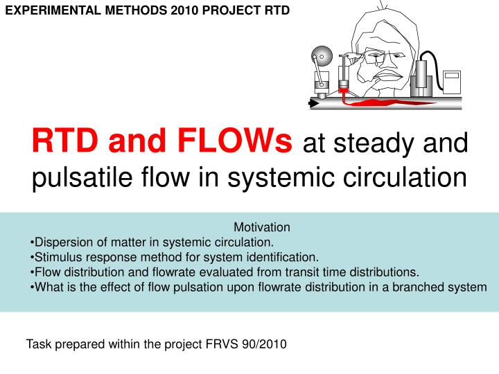
EXPERIMENTAL METHODS 2010 PROJECT RTD RTD and FLOWs at steady and pulsatile flow in systemic circulation Motivation Dispersion of matter in systemic circulation. Stimulus response method for system identification. Flow distribution and flowrate evaluated from transit time distributions. What is the effect of flow pulsation upon flowrate distribution in a branched system Task prepared within the project FRVS 90/2010
EXPERIMENTAL METHODS 2010 PROJECT RTD Residence times OUTLET INLET Fast particle (short residence time) Residence time = time spend by a particle inside a continuous system between inlet and outlet. RTD Residence time distribution E()= histogram of residence times of all particles passing through outlet. Applications of E(): Prediction of chemical reactions yield, transport of farmaceuticals, evaluation of active and stagnant volumes, diagnostics,… There are generally different RTDs for plasma and RTDs of blood particles. Different RTD exists at steady and pulsatile flow.
EXPERIMENTAL METHODS 2010 PROJECT RTD Unit IMPULSE stimulus OUTLET INLET All particles passing through inlet at time interval (tI,tI+dt)are marked “red” Stimulus response experiment E()=impulse response Experiments: “Red particles” – tracers (dyes, radionuclides, salts,…) are quickly injected to inlet. Detectors monitor concentration of tracer at outlet (impulse response). In our case the tracer is KCl solution and reflective particles injected from syringe, detectors are electric conductivity probes.
EXPERIMENTAL METHODS 2010 PROJECT RTD Response by Convolution Convolution enables to calculate response to an arbitrary stimulus function. It is possible to calculate impulse response E(t) by deconvolution from measured stimulus and response. cin(t), cout(t) concentration of tracer at inlet and outlet of a continuous system cin cout Convolution of stimulus and RTD function E Fourier transform of convolution t [s] Mean time of response = mean time of stimulus + mean residence time Variance of response = variance of stimulus + variance of E
EXPERIMENTAL METHODS 2010 PROJECT RTD RTD of pipe at convective regime Laminar flow and short residence times: diffusion can be neglected and residence times can be calculated from velocity field. The diffusion free regime is characterized by where Q-flow rate, L-pipe length, Dm-diffusion coefficient. Example: C~1000 at aorta, arteries, vena cava. Residence time distribution E() is the response to infinitely short impulse (delta function) cin E() cout Analytical solution exists also for response to a pulse of a finite width (violet line). Time of the first appearance is not affected, only mean response time is increased. (s) First appearance time =4s
EXPERIMENTAL METHODS 2010 PROJECT RTD Cresto Laboratory model of circulation Simulated part - pressure or conductivity transducers alternatively Platinum wires
EXPERIMENTAL METHODS 2010 PROJECT RTD NODES of simulation model Y [m] Data file defines the coordinates x,y,z of all 29 nodes 19 18 16 28 15 17 27 14 22 20 29 7 9 12 24 25 21 6 8 26 5 10 11 13 4 3 Conductivity probes. Q-flowrate, C-response (defined in form of table) 23 2 1 -0.4 -0.3 -0.2 -0.1 0 0.1 0.2 0.3 0.4 0.5 0.6 0.7 0.8 X [m]
EXPERIMENTAL METHODS 2010 PROJECT RTD ELEMENTS of simulation model V5(14,16,15,27,d3,d4,d4) V6(17,18,19,28,d3,d4,d4) V7(20,22,21,29,d3,d4,d4) P6(7,17,d3) P5(9,14,d3) P7(6,20,d3) V3(8,9,10,25,d2,d3,d3) 25 V2(5,6,7,24,d2,d3,d3) P4(8,11,d3) P3(4,8,d2) P2(3,5,d2) V4(11,12,13,26,d3,d4,d4) V1(2,3,4,23,d1,d2,d2) Nodal indices Data files define connectivity of PIPES (2-node elements) DIVISION (3-node elements) P1(1,2,d1)
EXPERIMENTAL METHODS 2010 PROJECT RTD RESPONSEs generated by PIPES x2,y2,z2 Q2 ,c2(t) d x1,y1,z1 ,Q1, c1(t) Convolution realized by FFT, and by inverse transformation.
EXPERIMENTAL METHODS 2010 PROJECT RTD RESPONSEs generated by WYES Given c1(t) x2,y2,z2 Q2,c2(t) x3,y3,z3 Q3,c3(t) Intermediate response d1 x4,y4,z4 final response x1,y1,z1, Q1,c1(t) It is alternatively possible to characterize the whole wye as a perfectly mixed vessel. In this case the both responses c3 and c2 will be identical PROBLEMS: 1. Derive impulse response of perfectly mixed vessel Emixed(t) 2. How to modify the responses in the case that detectors record not the tracer concentration but the flowrate of tracer (e.g. radiotracer – counter records rate of decays in the whole outlet).
EXPERIMENTAL METHODS 2010 PROJECT RTD Simulation in MATLAB MATLAB M-files available at http: • Simulation proceeds according to M-file RTD.m in steps • Reading input files xyzq,seq,cp,cv (txt) defining nodes, flowrate and elements • Definition of time scale, time steps, and stimulus function at entry node 1. • Evaluation of responses sequentially in all elements (sequence is defined in vector seq). Responses are evaluated by FFT in functions • function cout=convpipe(t,n,dt,cin,d,l,q) • tmean=pi*d^2*l/(4*q); • for i=1:n • if t(i)<tmean/2 • e(i)=0; • else • e(i)=tmean^2/(2*t(i)^3); • end • end • fcin=fft(cin); • fe=fft(e); • fcout=fcin.*fe; • cout=ifft(fcout)*dt; • end
EXPERIMENTAL METHODS 2010 PROJECT RTD Simulation in MATLAB MATLAB M-files available at http: Input data files: xyzq.txt x y z q (nodal coordinates and flowrates) seq.txt e1 e2 … (sequence of evaluated elements, +pipes, -wyes) cp.txt i j d (pipe -indices of nodes and diameter) cv.txt i j k l d1 d2 d3(wye - indices of nodes and diameters) TASK: 1. Modify input files according to parameters of your experiment 2. Compare calculated and measured concentration responses 3. Evaluate flowrates in branches from the shortest/mean transit times
EXPERIMENTAL METHODS 2010 PROJECT RTD Experiments: UVP velocities Ultrasound Doppler effect for measurement velocity profiles • Piezotransducer is transmitter as well as receiver of US pressure waves operating at frequency 4 or 8 MHz. • Short pulse of US waves is transmitted (repetition frequency 244Hz and more) and crystal starts listening received frequency reflected from particles in fluid. • Time delay of sampling (flight time) is directly proportional to the distance between transducer and the reflecting particle moving with the same velocity as liquid. • Received frequency differs from the transmitted frequency by Doppler shift Δf, that is proportional to the component of particle velocity in the direction of transducer axis. http://biomechanika.cz PROBLEMS: • What is spatial resolution of velocity, knowing speed of sound in water (1400 m/s) and sampling frequency 8 MHz ? • Calculate flowrate in a circular pipe from recorded velocity profile (given angle )
EXPERIMENTAL METHODS 2010 PROJECT RTD Experiments: flowrates • Flowrate can be identified also from the stimulus response experiments • Mean residence time • Shortest residence time (time of the first appearance) • Cross-correlation of stimulus and response functions http://biomechanika.cz
EXPERIMENTAL METHODS 2010 PROJECT RTD LABORATORY REPORT • Front page: Title, authors, date • Content, list of symbols • Introduction, aims of project, references • Description of experimental setup • Experiments with injection of tracer at a steady state regime. Record responses and pressures. • Evaluate flowrate from recorded pressure drop. Check Re and flow regime. • Evaluate flowrate from recorded responses and transit times. • Evaluate flowrate from velocity profiles recorded by UVP monitor. • Simulation (steady state). Modify input files and M-files according to measured flowrates and concentration profile at inlet. Evaluate theoretical responses at nodes with conductivity detectors. • Adjust flowrate pulsation and repeat tracer experiments. • Evaluate flowrate distribution at pulsatile flow and compare relative flowrates with steady state case. • Conclusion (identify interesting results and problems encountered)