Download
1 / 21
220 likes | 325 Views
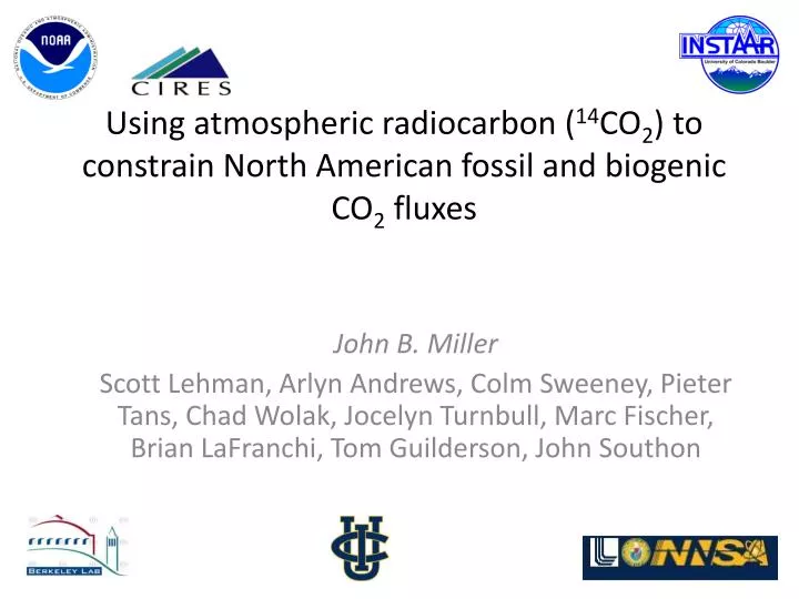
Using atmospheric radiocarbon ( 14 CO 2 ) to constrain North American fossil and biogenic CO 2 fluxes. John B. Miller Scott Lehman, Arlyn Andrews, Colm Sweeney, Pieter Tans, Chad Wolak , Jocelyn Turnbull, Marc Fischer, Brian LaFranchi , Tom Guilderson , John Southon.

E N D
Using atmospheric radiocarbon (14CO2) to constrain North American fossil and biogenic CO2 fluxes John B. Miller Scott Lehman, Arlyn Andrews, Colm Sweeney, Pieter Tans, Chad Wolak, Jocelyn Turnbull, Marc Fischer, Brian LaFranchi, Tom Guilderson, John Southon
Fossil Fuel are the biggest annual global and N. American fluxes… • …but, at many time scales NEE is bigger, which makes FF hard to identify (see Yoichi Shiga poster) • Inventories are good; why check them? • They have spatio-temporal biases at the state/monthly and smaller scales. • Generally, for up to date inversions, we need to extrapolate inventories. Global USA
Biases in FF will manifest themselves as biases in NEE in inversions, when using only CO2 • So, with a limited set of 14C observations, we’ll soon focus on relaxing the assumption of FF_error = 0. • Eventually, with more 14C observations, we’ll move towards direct emissions verification. • Here, I’ll describe our data and our modeling framework (and some examples of constraints of NEE and fossil fluxes).
14C is a theoretically robust tracer for fossil fuel fluxes. Total D14C looks just like fossil CO2. D14Cff = -1000 per mil (i.e. zero 14C) Scaling: -2.7 per mil D14C = 1 ppm CO2-fossil D14C Cff Catm*dDatm/dt = (Dfos-Datm)Ffos + DdisFsurf_gross+ isoFnuc+ isoFcosmo dCatm/dt = Ffos+ Fnet_surf + Ffire
Results of simulated 14CO2 inversions show Fossil Fuel emissions can be retrieved with low uncertainty NRC Recommendation of large increase in 14CO2 measurements to verify reductions 5000 measurements per year over the US (currently ~ 750) Monthly, state-sized fluxes at ~ 10% uncertainty.
Current network of sites samples a large fraction of N. American fossil fuel emissions. Dense enough to relax assumption of perfectly known fossil fuel emissions. (without sacrificing precision in NEE)
US PBL data show expected depletions of 14C(… AND enhancements of other anthropogenic gases: see Steve Montzka’s poster) NWR Downwind PBL 10 ppm Cff ~ 2-3 samples/week
CO2 PBL enhancements (or depletions) can be partitioned into NEE and Fossil fractions. PBL enhancement • Fossil Fuel masks Bio signal • Cbio large even in winter (~60% of total winter-time enhancement) despite urban/industrial observational footprint • CO2-only methods (tower, satellite, etc.) can not assume enhancements are due just to Cff US East Coast 300 m asl (see Miller et al, JGR-D 2012)
How well can we model our observations?(using TM5 with full 14CO2 and CO2 budget) Land (CASA model) Ocean (GLODAP/WOCE) TM5 Fluxes Concentrations Fossil (CDIAC/CT) Cosmogenic (50/50 Strat/trop) Nuclear Power (Graven)
The global trend and background for N. America are modeled very well. Bias = 0.8 per mil Stdev = 2.3 per mil
…And depletions relative to the trend fairly well. R2= 0.50 1:1
At polluted tower sites, seasonally varying depletion is captured. NWR • Seasonal cycles probably driven by wind direction co-varying with flux • (not PBL height or flux seasonality)
Downwind of mid-Atlantic East Coast, there are significant differences in vertical gradients
Vulcan’s emissions match data better because of lower urban emissions. Vulcan minus CT Standard CT-FF Vulcan FF
CMA(Vulcan fossil fuel emissions) But, Vulcan may still have too much FF fuel emission near the coast in urban areas.
Summary • 14CO2 can partition NEE and FF fluxes – AND CO2 ≠ Cff • Increasingly dense set of 14CO2 observations that will allow us to soon relax the assumption of fixed FF in inversions. • A reliable modeling framework. • Some ability already to distinguish fossil fuel patterns.
Detection Sensitivity allows for < 1ppm recently added Fossil Fuel CO2 NWT3 by measurement order: manual = 43.25 ± 1.60 Crex = 43.26 ± 1.65 Sigma-Cff = sqrt(2) * 1.8 per mil / 2.7 per mil/ppm = 0.9 ppm Determination of background is always important!
use of 14C + CO2 in CT to improve NEE CT 2000-10 Fffprior (given 0 uncertainty) NEE posterior retrieval deviation Fff prior from actuals will lead directly to bias in retrieved Fbio (NEE) from inversion of Cobs dCobs/dt = Fff + Fbio + Ffire Fff is large w.r.t net annual Fbio, and.. extrapolation of Fff inventories will not capture Fff anomalies associated with sustained heat and cold waves